( printed page 51856)

SUPPLEMENTARY INFORMATION:

Table of Contents

I. Introduction

II. Background on Stress Testing Framework, Stress Test Models, and Scenario Design Framework

A. Stress Testing Framework

B. Prior Supervisory Stress Disclosures and Policy Statements

C. Supervisory Stress Test Modeling Framework

D. Stress Test Models

E. Summary of the Proposal

F. Purpose of the Proposal

III. Overview of the Stress Test Modeling Framework

A. Supervisory Stress Test Models

B. Supervisory Stress Test Scenarios

C. Data Used in Stress Testing

IV. Enhanced Disclosure Process

A. Annual Disclosure of Models

B. Model Changes

C. Material Model Changes

D. Annual Disclosure of Scenarios

E. Stress Capital Buffer Requirement Reconsideration Process

V. Revisions to the Stress Testing Policy Statement

A. Future Supervisory Stress Test Results Disclosures

B. Other Revisions to the Stress Testing Policy Statement

VI. Other Revisions to the Stress Testing and Capital Plan Rules

A. Stress Test Jump-Off Date Change

B. Global Market Shock Date

C. Amendment to the Dividend Add-On Component Calculation

VII. Revisions to the FR Y-14A/Q/M

VIII. Proposed Changes to the Stress Test Modeling Framework

A. Proposed Changes to Stress Test Models

B. Analysis of Proposed Model Changes

IX. Proposed Changes to the Scenario Design Policy Statement

A. Changes to the Background and Overview and Scope Sections

B. Changes to the Content of the Stress Test Scenarios Section

C. Approach for Formulating Macroeconomic Assumptions in the Baseline Scenario

D. Scenario Narrative: Refinement to the Recession Approach

E. Changes to Construction of Certain Variables in the Severely Adverse Scenario

F. Scenario Design Principles Derived From Stress Testing Literature: Severity, Credibility, and Procyclicality

G. Description of Variable Guides in the Severely Adverse Scenario

H. Global Market Shock

X. Economic Analysis

XI. Administrative Law Matters

A. Paperwork Reduction Act Analysis

B. Regulatory Flexibility Act Analysis

C. Plain Language

D. Providing Accountability Through Transparency Act of 2023

I. Introduction

In December 2024, the Board announced that it would propose significant changes to improve the transparency of the supervisory stress test and reduce the volatility of resulting capital requirements.^[1] The Board noted it planned to propose changes to disclose and seek public comment on the models that determine the ( printed page 51857) hypothetical losses and revenue of banks under stress and ensure that the public can comment on the hypothetical scenarios used annually for the test, before the scenarios are finalized. With this proposal, the Board is inviting public comment on the comprehensive model documentation for the 2026 stress test, as well as proposed changes to the models relative to the 2025 stress test. The comprehensive model documentation is available at https://www.federalreserve.gov/​supervisionreg/​dfa-stress-tests-2026.htm. The Board is inviting comment on the proposed scenarios for the 2026 stress test through a separate notice.

This proposal seeks to improve the transparency and public accountability of the supervisory stress test, while ensuring that the stress test remains an effective tool for understanding and assessing risk and retaining appropriate risk sensitivity and risk capture in capital requirements.

The Board periodically reviews its regulations, including transparency efforts surrounding its regulations, to ensure they continue to achieve their goals in an effective and efficient manner. In addition to the changes discussed herein, the Board is also considering the effectiveness of its regulatory capital and capital planning requirements for large firms to ensure they remain cohesive and effective, maintain the resilience of the banking sector, and minimize any unnecessary burden. If appropriate, the Board will make changes to its rules through the public notice and comment process.

Question 1: The Board seeks comment on all aspects of the proposal. What, if any, other elements of the supervisory stress test framework should the Board consider amending to improve the transparency, public accountability, and effectiveness of the supervisory stress test? For example, the Board could instead transliterate the models used to conduct the stress test and codify these transliterations in its regulations. What would be the advantages and disadvantages of this approach or other approaches the Board could consider?

II. Background on Stress Testing Framework, Stress Test Models, and Scenario Design Framework

A. Stress Testing Framework

Congress enacted the Dodd-Frank Wall Street Reform and Consumer Protection Act (Dodd-Frank Act) in the wake of the 2007-09 financial crisis.^[2] Section 165 of the Dodd-Frank Act, as amended by section 401 of the Economic Growth, Regulatory Relief, and Consumer Protection Act,^[3] requires the Board to establish enhanced prudential standards for nonbank financial companies supervised by the Board and bank holding companies with $250 billion or more in total consolidated assets.^[4] The purpose of these enhanced prudential standards is to prevent or mitigate risks to the financial stability of the United States that could arise from the material financial distress or failure, or ongoing activities, of large, interconnected financial institutions.

Section 165(i)(1) of the Dodd-Frank Act requires the Board to conduct an annual supervisory stress test of nonbank financial companies supervised by the Board and bank holding companies with $250 billion or more in total consolidated assets to evaluate whether the firm has the capital, on a total consolidated basis, necessary to absorb losses as a result of adverse economic conditions.^[5] Section 401(e) of the Economic Growth, Regulatory Relief, and Consumer Protection Act requires the Board to conduct periodic stress tests for bank holding companies with total consolidated assets between $100 billion and $250 billion.^[6] Section 165(i)(1) of the Dodd-Frank Act requires the Board to publish a summary of the supervisory stress test results.^[7] In 2012, the Board adopted a final rule implementing the stress test requirements established in the Dodd-Frank Act.^[8]

The Dodd-Frank Act also requires bank holding companies with $250 billion or more in total consolidated assets, as well as nonbank financial companies supervised by the Board, to conduct company-run stress tests on a periodic basis.^[9] Under the Board's rules, firms subject to Category I, II, or III standards must conduct company-run stress tests.^[10] Company-run stress tests provide forward-looking information to supervisors to assist in their overall assessments of a firm's capital adequacy, help to better identify downside risks and the potential impact of adverse outcomes on the firm`s capital adequacy, and assist in achieving the financial stability goals of the Dodd-Frank Act. Further, the company-run stress tests help improve firms' stress testing practices with respect to their own internal assessments of capital adequacy and overall capital planning.

Each June, the Board publishes the results of its annual supervisory stress test, including each firm's projected capital ratios, pre-tax net income, losses, revenues, and expenses, under hypothetical, severely adverse economic and financial conditions.^[11] These disclosures provide the public with valuable information about each firm's financial condition and the ability of ( printed page 51858) each firm to absorb losses considering a stressful economic environment.

Following the 2007-09 financial crisis, the Board also made changes to its capital rule to address weaknesses observed during the crisis.^[12] These changes included the establishment of a minimum common equity tier 1 capital requirement and a fixed capital conservation buffer equal to 2.5 percent of risk-weighted assets.^[13] Large firms also became subject to a countercyclical capital buffer requirement, and the largest and most systemically important firms—global systemically important bank holding companies, or GSIBs—became subject to an additional capital buffer based on a measure of their systemic risk, the GSIB surcharge.^[14] In 2020, the Board adopted the stress capital buffer requirement for certain firms.^[15] Because a firm's stress capital buffer requirement is informed by the firm's performance under the hypothetical economic conditions modeled by the supervisory stress test, each firm's stress capital buffer requirement is tailored to its risk profile.

Supervisory stress testing and stronger capital requirements have significantly improved the resilience of the U.S. banking system. Since 2009, the common equity capital ratios of firms subject to the test have more than doubled, with common equity capital of such firms increasing by over $1 trillion.^[16] Since 2020, the supervisory stress test results have also informed a firm's stress capital buffer requirement. Greater transparency would allow firms to better understand the capital requirements associated with investment and expansion of different business lines and would facilitate more effective long-term capital planning. This, in turn, could enhance firms' ability to supply credit to households and businesses, ultimately supporting economic growth and financial stability.

B. Prior Supervisory Stress Disclosures and Policy Statements

In addition to the annual stress test results disclosure, the Board has historically published some information about the supervisory stress test scenarios and models.

Scenarios

The Board's stress test rules provide that the Board will notify firms, by no later than February 15 of each year, of the scenarios that the Board will apply to conduct its annual supervisory stress test and that firms must use to conduct their company-run stress tests.^[17] The Board also provides a narrative description of the scenarios no later than February 15 of each calendar year.^[18]

In 2013, the Board increased the transparency of the scenarios by finalizing the Policy Statement on the Scenario Design Framework for Stress Testing (Scenario Design Policy Statement), which articulated the Board's approach to scenario design for the supervisory and company-run stress tests, outlining the characteristics of the stress test scenarios, and explaining the considerations and procedures that underlie the formulation of these scenarios.^[19] The Scenario Design Policy Statement also described the baseline and severely adverse scenarios, the Board's approach for developing these two macroeconomic scenarios, and the approach for developing any additional components of the stress test scenarios. The Scenario Design Policy Statement explained that the severely adverse scenario is designed to reflect conditions that have characterized post-war U.S. recessions (the recession approach). Historically, recessions have typically featured increases in the unemployment rate, contractions in aggregate incomes and economic activity, and declines in inflation and interest rates.

In the 2013 Scenario Design Policy Statement, the Board explained that, in light of the typical co-movement of measures of economic activity during economic downturns, such as the unemployment rate and gross domestic product, the Board would first specify a path for the unemployment rate and then develops paths for other measures of activity broadly consistent with the course of the unemployment rate in developing the severely adverse scenario. The 2013 Scenario Design Policy Statement also stated that economic variables included in the scenarios may change over time, and that the Board may augment the recession approach with certain salient risks, which would involve incorporating features that address aspects of the current economic or financial market environment that represent higher-than-normal risks to the condition of the banking system.

In 2019, the Board updated the Scenario Design Policy Statement, which increased the transparency and predictability of the scenarios by allowing for a smaller-than-usual increase in unemployment if the stress test were to occur during an economic downturn, a change that would pass through to reduced severity of other key scenario variables due to the deference given to historical correlations. The 2019 update also introduced a formula with countercyclical features to guide the evolution of the ratio of housing prices to disposable income in the scenario, which provided more predictability in the way that the stress test would treat business lines affected by changes in house prices. However, the Board believes that the design of scenarios could be made more transparent and predictable by providing additional guides for certain macroeconomic variables, and by disclosing additional detailed information on the methodology used to create the global market shock component of the severely adverse scenario, as described below.

a. Trading and Counterparty Components

For a subset of firms, the severely adverse scenario also includes two additional components: the global market shock component and the largest counterparty default component.^[20] The global market shock component is a set of hypothetical shocks to a large set of risk factors reflecting general market distress and heightened uncertainty. A firm with significant trading activity must consider the global market shock component as part of its severely adverse scenario and recognize associated losses in the first quarter of the projection horizon.^[21] The global ( printed page 51859) market shock component is applied to asset positions held by the firms on a given as-of date.^[22] In addition, for certain large and highly interconnected firms, the same global market shock component is applied to counterparty exposures under the largest counterparty default component.^[23] The largest counterparty default component is intended to assess the potential losses and capital impact associated with the default of the largest counterparty of each applicable firm, and the as-of date aligns with that of the global market shock component.

The design and specification of the global market shock component differs from the design and specification of the severely adverse scenario in several respects. First, in alignment with U.S. generally accepted accounting principles (U.S. GAAP), profits and losses from trading and counterparty credit positions are measured in mark-to-market accounting terms in the global market shock, while revenues and losses from traditional banking activities, as generated under macroeconomic scenarios, are generally measured using the accrual accounting method. Second, the timing of loss recognition differs between the global market shock and the severely adverse macroeconomic scenario. The global market shock affects the mark-to-market value of trading positions and counterparty credit losses in the first quarter of the severely adverse scenario. This timing is based on an observation that market dislocations can happen rapidly and unpredictably at any time under stressed conditions. In addition, the severely adverse scenario is applied as of December 31 of each year (the jump-off date), whereas the global market shock as-of date changes every year (within the window specified in the Board's stress test rules) and does not necessarily coincide with the year-end. This timing is also based on a scenario assumption that market dislocations can happen rapidly and unpredictably at any time during the scenario horizon. Recognizing the global market shock in the first quarter helps ensure that potential losses from trading and counterparty exposures are incorporated into firms' capital ratios in each quarter of the severely adverse scenario.

Models

Prior to 2019, the annual stress test results disclosure document contained an appendix describing the Board's supervisory stress test models.^[24] In 2019, the Board increased the transparency of the supervisory stress test models by finalizing the Stress Testing Policy Statement ^[25] and the Enhanced Disclosure of the Models Used in the Federal Reserve's Supervisory Stress Test (Enhanced Model Disclosure).^[26] The Stress Testing Policy Statement describes the Board's policies and procedures that guide the development, implementation, and validation of the models.^[27] The Stress Testing Policy Statement also describes the Board's principles for stress test model design, namely that the system of models used in the supervisory stress test should result in projections that are (1) independent of firm projections; (2) forward-looking in that they project future losses and revenue; (3) consistent and comparable across firms; (4) generated from simple approaches, where appropriate; (5) robust and stable; (6) conservative; and (7) able to capture the effect of severe economic stress. The Board has developed stress test models in accordance with these principles, which are the foundation for the stress test modeling decisions described in the comprehensive documentation of the supervisory stress test models that the Board is publishing in conjunction with this proposal.

The Enhanced Model Disclosure supplemented prior public descriptions of the stress test models by providing some information about their structure and by including a list of key variables that influence the results of each model.^[28] However, the Board believes more detailed information, beyond what is in the current Enhanced Model Disclosure, would improve the ability of firms to accurately assess how changes in their business activities might impact their supervisory stress test results and, relatedly, their stress capital buffer requirements and overall capital requirements.

C. Supervisory Stress Test Modeling Framework

The Board's stress test models take macroeconomic variables from the Board's severely adverse scenario and firm data as inputs to produce each firm's projected capital ratios over a nine-quarter horizon. The projected common equity tier 1 capital ratio is used to inform each firm's stress capital buffer requirement, which becomes part of a firm's capital conservation buffer.

The stress test models are intended to capture how a firm's regulatory capital would be affected by the macroeconomic and financial conditions described in the stress test scenarios, given the characteristics of the firm's business model and balance sheet composition. The Board uses a variety of statistical modeling techniques to produce the stress test results, including multivariate regression, which uses relationships in historical data to produce projections of a variable (such as a loss given default). These models are represented by a set of formulas and coefficients that produce the projections.

The Board estimates the effect of the severely adverse scenario on the regulatory capital ratios of firms by projecting revenues, expenses, and losses for each firm over a nine-quarter projection horizon (projection horizon). The projection horizon spans nine quarters to ensure that the firms can continue to provide credit and serve as financial intermediaries despite several quarters of adverse economic conditions, as well as to promote the forward-looking nature of capital planning by firms.

Projected net income, adjusted for the effect of taxes, is combined with assumptions regarding capital actions and other changes to regulatory capital to produce post-stress capital ratios. The Board's approach to modeling supervisory stress test results, including the calculation of post-stress capital ratios, is generally in alignment with U.S. GAAP and the regulatory capital framework.^[29] However, the stress test models may deviate from U.S. GAAP and the regulatory capital framework, as circumstances warrant.

The Board established the Stress Testing Policy Statement modeling principles to ensure that the models are well suited for their purpose in the regulatory framework. In some cases, the Board's adherence to the principles limits modeling choices and results in certain common limitations across similarly constructed component ( printed page 51860) models. For instance, consistent with the principles of independence, consistency and comparability, and simplicity, models are not designed to capture all firm-specific nuances, future strategic initiatives, or planned capital actions. Additionally, models may be limited by their reliance on historic relationships and by the nature of the data captured in firms' regulatory reports. Detailed assumptions and limitations for the models are discussed in the comprehensive documentation, which is available at https://www.federalreserve.gov/​supervisionreg/​dfa-stress-tests-2026.htm.

Under the Stress Testing Policy Statement, the Board's projections also assume that a firm's balance sheet remains unchanged throughout the projection horizon.^[30] This assumption seeks to help ensure that a firm cannot “shrink to health” and that it remains sufficiently capitalized to accommodate credit demand in a severe downturn.

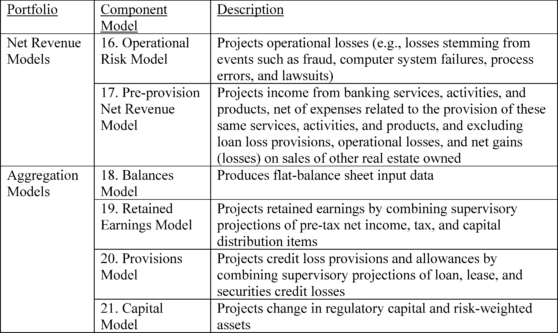
D. Stress Test Models

The Board's stress test models comprise twenty-one component models that, when aggregated, produce projected regulatory capital ratios for each firm (see Table 1 below). The models can be grouped into four categories: credit risk, market risk, net revenue, and aggregation. Credit risk models capture losses associated with retail and wholesale loans that are held at amortized cost. Market risk models capture losses associated with trading and counterparty exposures, securities, and other assets held at fair value. Net revenue models capture income and expenses, including those related to operational risk, earned or incurred by a firm. Positive pre-provision net revenue offsets credit and market risk losses in the calculation of a firm's pre-tax net income. Aggregation models calculate a firm's pre-tax net income, which is then adjusted for other elements such as taxes and regulatory capital deductions to arrive at the projection of a firm's regulatory capital, which is used to calculate a firm's projected capital ratios. Additional detail about these component models is provided in Section III.A of this Supplementary Information and the comprehensive model documentation available at https://www.federalreserve.gov/​supervisionreg/​dfa-stress-tests-2026.htm.^[31]

( printed page 51861)

( printed page 51862)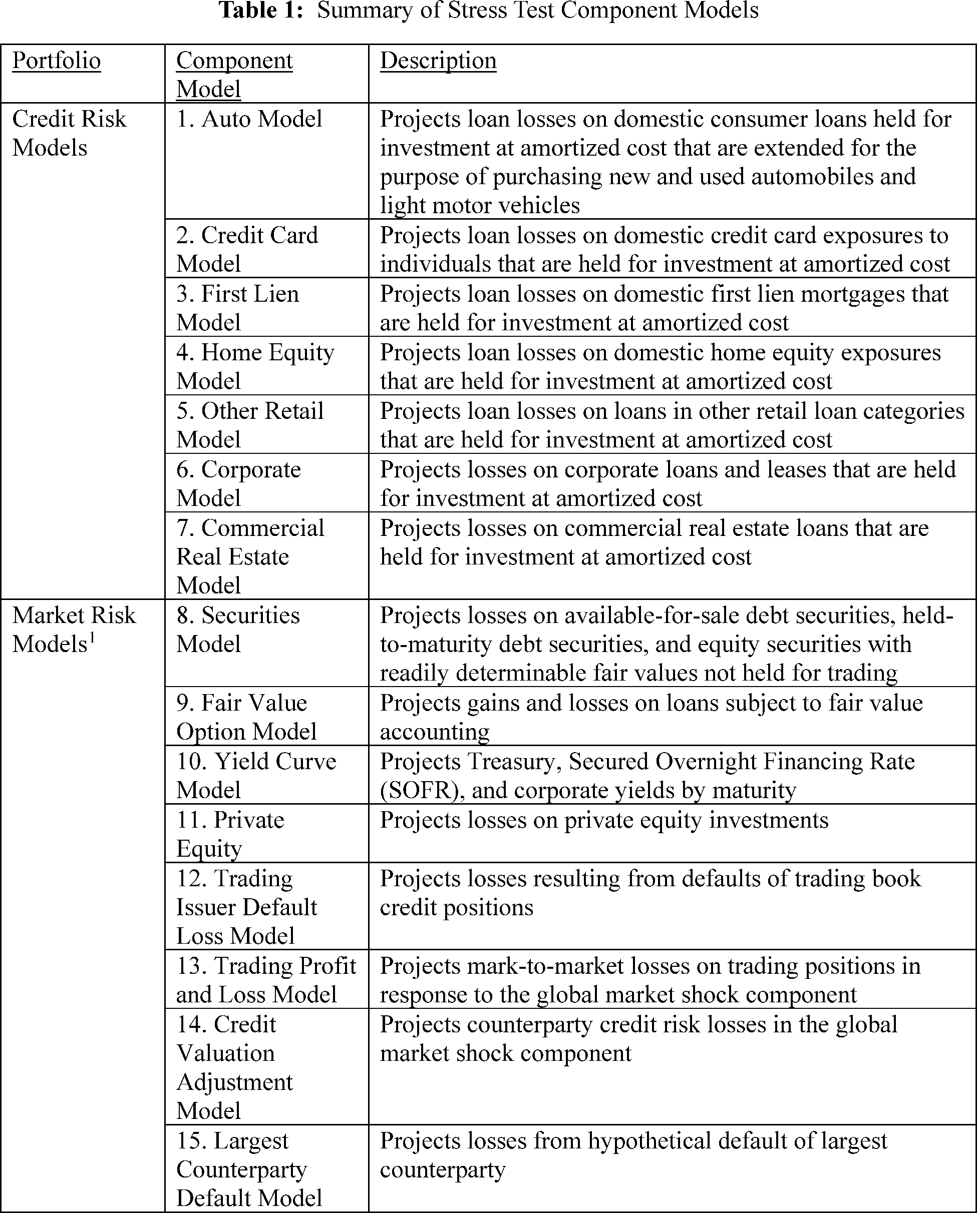

E. Summary of the Proposal

The Board is publishing comprehensive documentation on the stress test models on the Board's website, at https://www.federalreserve.gov/​supervisionreg/​dfa-stress-tests-2026.htm. This model documentation contains information on the models that together produce the results of the supervisory stress test. The model documentation includes the equations, variables, and coefficients used in each model (where applicable); assumptions and limitations of each model; rationales for modeling decisions; and discussions of alternative models. Section VIII.A of this Supplementary Information summarizes changes to the models, relative to the 2025 stress test, that the Board plans to implement in the 2026 stress test cycle; section VIII.B of this Supplementary Information contains an analysis of the potential effects of these proposed model changes. Detailed documentation on these changes is also provided on the Board's website, at https://www.federalreserve.gov/​supervisionreg/​dfa-stress-tests-2026.htm. As part of this proposal, the Board is inviting public comment on the stress test models and these changes.

In addition, the Board is proposing to codify an enhanced disclosure process that would build on the previous efforts that the Board has made to increase the transparency and public accountability of the supervisory stress test. Under this enhanced disclosure process, the Board would annually publish comprehensive model documentation on the stress test models, invite public comment on any material changes that the Board seeks to make to those models, and annually publish the stress test scenarios for comment. The Board would also commit to responding to substantive public comments on any material model changes before implementing them. The proposal would revise the Stress Testing Policy Statement to align with this enhanced disclosure process, as well as to amend the Board's general policy related to disclosing additional information directly to a firm about that firm's supervisory stress test results. To accommodate the annual comment process on the scenarios, the proposal would shift the jump-off date of the supervisory and company-run stress tests from December 31 to September 30.

Additionally, this proposal would amend the Scenario Design Policy Statement in several ways. The Board would include in the Scenario Design Policy Statement detailed descriptions of additional guides that are used to inform the Board's choice of the values of the scenario variables along their scenario paths. The guides are designed to balance the competing objectives of predictability and transparency, on the one hand, with the severity and relevance of the macroeconomic and financial market scenarios, on the other hand. Most of the proposed guides also incorporate features similar to the range of options in the existing unemployment guide or the automatic adjustment of the house price path to current housing market conditions in the existing house price guide. This approach would allow the Board to continue to adjust the severity of those variables as necessary to avoid inducing greater procyclicality in the financial system and macroeconomy.

Similarly, the Board is proposing to incorporate additional information into the Scenario Design Policy Statement about the framework used to create the global market shock component of the severely adverse scenario. This information includes, but is not limited to, details on the logic underlying the severity of the shocks and a description of the processes used to generate the shock values. The Board is also proposing to update the global market shock methodology to simplify the scenario and better align certain elements of the global market shock with the nature of an “instantaneous” shock. The proposal would also make revisions to the stress test rules to improve the risk capture of the supervisory stress test by widening the ( printed page 51863) as-of date window for the global market shock.

Finally, the proposal would make changes to the FR Y-14A/Q/M reports to remove items and documentation requirements that are no longer needed to conduct the supervisory stress test, as well as to collect additional data to improve risk capture.

F. Purpose of the Proposal

The purpose of this proposal is to provide the public with more information about the stress test models and scenarios and to help ensure that the public has an opportunity to comment on the models and scenarios. While the Board has increased the transparency of the stress test models over time, disclosing additional information about the stress test models and their underlying methodologies will further increase transparency and improve public accountability.

Publishing detailed descriptions of the stress test models for comment, as well as committing to future enhanced disclosures, has benefits. First, the increase in transparency would increase public accountability and instill confidence in the fairness of the supervisory stress tests. Second, the disclosure process would create a new mechanism for obtaining feedback from the public, including academics, financial analysts, and firms, on the design and specifications of the models, which should lead to model improvements. Third, a firm would have a better sense of how its risk profile would factor into its stress capital buffer requirement, which would reduce the likelihood of unanticipated stress test results and allow for better capital and business planning by firms. Finally, the public disclosure of additional information about supervisory stress tests should strengthen market discipline, because investors, counterparties, and rating agencies would be able to better assess a firm's risk profile.^[33] The costs and benefits of this proposal are described more thoroughly in Section X of this Supplementary Information.

With respect to the proposed amendments to the Scenario Design Policy Statement, this proposal also builds on the contents of the current Scenario Design Policy Statement and would amend it to provide additional transparency, public accountability, and predictability in the variable paths. The changes would support the Board in developing scenarios, inviting comment on those scenarios, incorporating input from commenters, and maintaining the current schedule for release of the final scenarios. Despite the increased predictability in the scenarios, the new framework would remain flexible enough to suitably assess whether firms can maintain an adequate amount of loss-absorbing capital to stay above minimum regulatory requirements and continue financial intermediation during periods of stress, as well as adjust features that might add to existing procyclicality in the financial system, as appropriate. In practice, the scenarios resulting from the revised framework are expected to remain consistent with the current Scenario Design Policy Statement and should not result, on average over a typical business cycle, in materially different scenarios than would have been designed previously.

Additionally, the proposal would simplify the design of the global market shock component and incorporate additional information on the development process into the Scenario Design Policy Statement, which outlines the Board's approaches to designing market shocks, including important considerations for scenario design, possible approaches to developing scenarios, and a development strategy for implementing the preferred approach. Taken together, these changes would improve transparency, public accountability, and predictability of the supervisory scenarios, while ensuring the supervisory stress test's ability to capture changes in the risks in the financial industry over time.

III. Overview of the Stress Test Modeling Framework

As summarized in Section II.D of this Supplementary Information, the Board estimates the effect of the scenarios on the regulatory capital ratios of firms participating in the stress test by projecting net income and other components of regulatory capital for each firm over a nine-quarter projection horizon. To do so, the Board uses twenty-one component models, the macroeconomic variables from the Board's severely adverse scenario, and firm data. This section provides an overview of the component models the Board used to run the 2025 supervisory stress test. See Table 1 in Section II.D of this Supplementary Information.

A. Supervisory Stress Test Models

The Board calculates projected pre-tax net income by combining projections of pre-provision net revenue,^[34] provisions for credit losses,^[35] and other gains or losses.^[36] Each component of pre-tax net income is described below.

Pre-Provision Net Revenue

Pre-provision net revenue is defined as net interest income (interest income minus interest expense) plus noninterest income minus noninterest expense. Consistent with U.S. GAAP, these projections include projected losses due to operational risk events and expenses related to the disposition of other real estate owned.^[37] The Board projects most components of pre-provision net revenue using models that relate specific revenue and non-provision-related expenses to the characteristics of firms and to macroeconomic variables. These include eight components of interest income, seven components of interest expense, six components of noninterest income, and three components of noninterest expense. The Board separately projects losses from operational risk and other real estate owned expenses. Operational risk is defined as “the risk of loss resulting from inadequate or failed internal processes, people and systems or from external events.” ^[38] Other real estate owned expenses are expenses related to the disposition of real estate owned properties and stem from losses on first-lien mortgages.

Loan Losses and Provisions on Loans Measured at Amortized Cost

The Board typically projects losses using one of two modeling approaches: the expected-loss approach or the net charge-off approach. Generally, under the expected loss approach, expected losses are estimated by projecting the probability of default, loss given default, and exposure at default for each quarter of the projection horizon. Expected losses in each quarter are the product of these three components. Under the net ( printed page 51864) charge-off approach, losses are projected using historical behavior of net charge-offs as a function of macroeconomic and financial market conditions and loan portfolio characteristics.^[39]

The Board estimates losses for loans measured at amortized cost separately for different categories of loans, based on the type of obligor, collateral, and loan structure. The individual loan types modeled can broadly be divided into (1) retail loans, including various types of residential mortgages, credit cards, student loans, auto loans, small business loans, and other consumer loans; and (2) wholesale loans, such as commercial and industrial loans and commercial real estate loans. For most loan types, losses in quarter t are estimated as the product of the projected probability of default in quarter t, the loss given default in quarter t, and exposure at default in quarter t.

The probability of default component measures the likelihood that a borrower enters default status during a given quarter t. The other two components capture the lender's net loss on the loan if the borrower enters default. The loss given default component measures the percentage of the loan balance that the lender will not be able to recover after the borrower enters default, and the exposure at default component measures the total expected outstanding loan balance at the time of default.^[40]

The Board's definition of default, for stress test modeling purposes, may vary for different types of loans and may differ from general industry definitions or classifications. The Board generally models probability of default as a function of loan characteristics and economic conditions. The Board typically models loss given default based on historical data, and modeling approaches vary for different types of loans. For certain loan types, the Board models loss given default as a function of borrower, collateral, or loan characteristics and the macroeconomic variables from the supervisory scenarios. For other loan types, the Board assumes loss given default is a fixed percentage of the loan balance for all loans in a category. The approach to modeling exposure at default also varies by loan type and depends on whether the loan is a term loan or a line of credit.

For certain retail loan categories, projections capture the historical behavior of net charge-offs as a function of macroeconomic and financial market conditions and loan portfolio characteristics. The Board then uses these stress test models to project future charge-offs consistent with the evolution of macroeconomic conditions under the severely adverse scenario. To project losses, the projected net charge-off rate is applied to projected loan balances.

Losses on loans are then projected to flow into net income through provisions for loan and lease losses (for simplicity, provisions for loan losses). Provisions for loan losses reflect funds set aside to cover loan losses that a firm expects to incur in a predetermined future window. Provisions for loan losses feed into the allowance for loan losses, which serves as a contra asset on a firm's balance sheet. The charged-off amount of a loan reduces the outstanding balance of the loan while also reducing the allowance for loan losses (that is, charge-offs do not reduce a firm's total assets). Generally, provisions for loan losses for each projected quarter in the supervisory stress test equal projected losses on loans for the quarter plus the change in the allowance for loan losses needed to cover the subsequent four quarters of expected loan losses. This calculation incorporates the allowance for loan losses established by the firm as of the jump-off date of the stress test exercise.

Current Expected Credit Losses Framework

On January 1, 2020, most large and mid-sized U.S. banks adopted the Current Expected Credit Losses (CECL) standard for calculating allowances.^[41] CECL superseded the incurred loss accounting standard, which was a backward-looking measure that enabled firms to calculate allowances based on historical loss data and current economic conditions. CECL, by contrast, is a forward-looking measure that requires firms to estimate lifetime losses based on reasonable estimates of future economic conditions. In October 2024, the Board announced that it would continue to evaluate future enhancements to the supervisory stress test approach for the incorporation of CECL.^[42]

The Board is not proposing to implement CECL into the supervisory stress testing framework as a part of this proposal. The allowance calculation framework currently used in the supervisory stress test is already forward-looking: it projects loan loss provisions four quarters ahead. This approach aligns with the Board's modeling principle of simplicity as it requires fewer assumptions than would be required to determine provisions under CECL. In addition, in aggregate, the cumulative loan loss provisions under the supervisory severely adverse scenario are similar to provision projections submitted by the firms that have adopted CECL. Should the Board decide to implement CECL into the supervisory stress testing framework, it would seek public comment prior to implementation, as it would likely be a material model change as defined in this proposal.

Question 2: What factors should the Board consider when determining whether to implement CECL into the supervisory stress testing framework and why?

Question 3: What would be the advantages and disadvantages of incorporating CECL into the supervisory stress testing framework?

Losses on Loans Measured on a Fair Value Basis

Certain loans are accounted for on a fair value basis instead of on an amortized cost basis. If a loan is accounted for using the fair value option, it is marked to market, and the accounting value of the loan changes as a function of changes in market risk factors and fundamentals. Similarly, loans that are held for sale are accounted for at the lower of cost or market value. The stress test models for these asset classes project gains and losses over the nine-quarter projection horizon, net of any hedges, using the scenario-specific path of interest rates and credit spreads. The Board uses different models to estimate gains and losses on wholesale loans and retail loans that are accounted for on a fair value basis since these loans have different risk characteristics. However, these models all generally project gains and losses over the nine-quarter projection horizon, net of hedges, by applying the scenario-specific interest rate and credit spread shocks to loan yields.

Losses on Securities

A firm's balance sheet typically contains holdings of two types of securities related to investment activities: available-for-sale and held-to- ( printed page 51865) maturity. Available-for-sale and held-to-maturity securities are generally held at fair value and amortized cost, respectively, on a firm's balance sheet. The Board estimates two types of losses on securities related to investment activities.^[43]

For debt securities classified as available-for-sale, projected fluctuations in the fair value of the securities due to changes in interest rates and other factors will result in unrealized gains or losses that are recognized in capital for some firms through other comprehensive income. Under U.S. GAAP, unrealized gains and losses on available-for-sale debt securities are reflected in accumulated other comprehensive income and do not flow through net income.^[44] Under the regulatory capital rule, accumulated other comprehensive income must be incorporated into common equity tier 1 capital for certain firms. Unrealized gains and losses are calculated as the difference between each security's fair value and its amortized cost. The amortized cost of each available-for-sale debt security is equivalent to the purchase price of the debt security, which is periodically adjusted if the debt security was purchased at a price other than par or face value, has a principal repayment, or has an impairment recognized in earnings.^[45]

Credit losses on available-for-sale and held-to-maturity securities may be also recorded. Except for certain government-backed obligations, both available-for-sale and held-to-maturity securities are at risk of incurring credit losses.^[46] The stress test models project security-level credit losses, using as an input the projected fair value for each security over the nine-quarter projection horizon under the severely adverse scenario. Credit losses on securities are included in the projection of provisions.

Projected other comprehensive income gains or losses from available-for-sale debt securities are computed directly from the projected change in fair value, taking into account credit losses and applicable interest-rate hedges on securities. All debt securities held in the available-for-sale portfolio are subject to other comprehensive income losses.

Losses on Private Equity Exposures

The Board projects the value of private equity investments in response to the severely adverse scenario of the supervisory stress test.^[47] The Private Equity Model assigns losses and recoveries based on changes in fair value, recognized in net income for all positions, regardless of their individual accounting elections. While U.S. GAAP allows for private equity to be carried under a variety of accounting measures, the different accounting methods are generally not reflective of fundamental risk differences—fair value is typically realized upon the orderly sale of a given private equity investment, irrespective of its accounting treatment during the holding period.^[48]

Losses on Trading Exposures

The trading stress test models cover a wide range of a firm's exposure to asset classes such as public equity, foreign exchange, interest rates, commodities, securitized products, traded credit (for example, municipal securities, auction rate securities, corporate credit, and sovereign credit), and other fair-value assets. Loss projections are constructed by applying the market risk factor movements specified in the global market shock component ^[49] to market values of firm-provided positions and risk factor sensitivities.^[50] The global market shock only applies to a subset of firms, as described in Section II.B.a of this Supplementary Information. In addition, the global market shock component is applied to firm counterparty exposures to generate losses due to changes in credit valuation adjustment, which is a change to the market value of an exposure (for example, a derivative) to account for the risk that the counterparty defaults on its obligation. Trading and credit valuation adjustment losses are calculated only for firms subject to the global market shock component. In contrast to the nine-quarter evolution of losses for other parts of the supervisory stress test, and as previously described, these losses are estimated and applied in the first quarter of the projection horizon. This timing is based on the observation that market dislocations can happen rapidly and unpredictably any time under stress conditions. It also ensures that potential losses from trading and counterparty exposures are incorporated into a firm's capital ratio at all points in the projection horizon.

The Board separately estimates the risk of losses arising from the default of issuers of debt securities held for trading. These losses account for concentration risk in corporate, sovereign, agency, and municipal credit positions. In contrast to the trading losses described above, these losses are applied in each of the nine quarters of the projection horizon to capture the risk that several quarters of stressful economic conditions may cause additional issuers of debt securities to default, which aligns with the Board's principle of conservatism from the Stress Testing Policy Statement.

Largest Counterparty Default Losses

The largest counterparty default component is applied to firms with substantial trading or custodial operations. This component captures the risk of loss due to the unexpected default of the counterparty whose default on derivatives and securities financing transactions, with exposures revalued by applying the global market shock component, would generate the largest stressed losses for a firm. Consistent with the Board's modeling principles and with the losses associated with the global market shock component, losses associated with the largest counterparty default component are recognized in the first quarter of the projection horizon.

Balance Projections and the Calculation of Regulatory Capital Ratios

As described above, the Board assumes that a firm takes actions to maintain its current level of assets, including its investment securities, trading assets, and loans, over the ( printed page 51866) projection horizon. The Board also assumes that a firm's risk-weighted assets and leverage ratio denominators remain unchanged over the projection horizon, except that the Board will account for changes primarily related to the calculation of regulatory capital or due to changes to the Board's regulations.^[51]

The Board includes five regulatory capital ratios in the supervisory stress test: (1) common equity tier 1 risk-based capital, (2) tier 1 risk-based capital, (3) total risk-based capital, (4) tier 1 leverage, and (5) supplementary leverage. A firm's post-stress regulatory capital ratios are projected in accordance with the Board's regulatory capital rule using the Board's projections of pre-tax net income and other scenario-dependent components of the regulatory capital ratios. Pre-tax net income and the other scenario-dependent components of the regulatory capital ratios are combined with additional information, including assumptions about taxes and capital distributions, to project post-stress measures of regulatory capital. In those calculations, the Board adjusts pre-tax net income to account for taxes and other components of net income, such as income attributable to minority interests, to arrive at after-tax net income. The Board calculates the change in equity capital over the projection horizon by combining projected after-tax net income with changes in other comprehensive income, assumed capital distributions, and other components of equity capital. The path of regulatory capital measures over the projection horizon is calculated by combining the projected change in equity capital with the firm's starting capital position and accounting for other adjustments to regulatory capital specified in the Board's regulatory capital framework.^[52] The denominator of each firm's risk-based capital ratios is based on a firm's standardized approach for calculating risk-weighted assets on the jump-off date of the supervisory stress test, and may change for each quarter of the projection horizon to account for adjustments specified in the capital rule (for example, adjustments due to the thresholds for deducting certain deferred tax assets).

B. Supervisory Stress Test Scenarios

The Board conducts the supervisory stress test using two scenarios—the baseline and severely adverse. The severely adverse scenario describes a hypothetical set of conditions designed to assess the strength and resilience of firms in a severely adverse economic environment and includes 28 variables that are disclosed by the Board each year prior to the supervisory stress test. Some variables describe economic developments within the United States while others describe developments in foreign countries.^[53] These variables serve as an input to the calculation of supervisory stress test results for all firms. As discussed above, for a subset of firms, the severely adverse scenario also includes two additional components: the global market shock component and the largest counterparty default component. The scenarios and associated components are developed solely for supervisory stress testing purposes and do not represent economic forecasts of the Board.

Geographic Variation of Macroeconomic Variables

While the Board projects the paths of macroeconomic variables at the national level, the Board uses regional-level (that is, state- and/or county-level) macroeconomic variables in the stress test models to project losses on certain loans held for investment at amortized cost.^[54] In general, model outputs are demonstrably impacted by the macroeconomic environment, as both probability of default and loss given default increase during periods of economic stress. Importantly, the macroeconomic environment can also vary notably across geography, in addition to across time. For instance, during the 2007-2009 crisis period, housing prices fell more sharply in certain geographies compared to others. Accordingly, historical loss rates in many loan categories were higher during this period in geographies where housing prices fell more sharply.

Therefore, to account for the impacts of different macroeconomic environments across geographies on historical loan performance, the Board calibrates model parameters in certain stress test models using regional macroeconomic variables as opposed to national macroeconomic variables. For example, the unemployment rate used in an applicable model may be the state level unemployment rate, while the house price index values used in the model may be the county-level house price indices or, in the case of loans in counties where a house price index is not projected, a state-level house price index.^[55] Analysis performed by the Board demonstrates that a certain model's statistical fit and sensitivity to the macroeconomic environment may perform better when using regional-level variables compared to when using only national-level variables. The use of regional-level variables is described in each applicable model section of the comprehensive model documentation.

However, because the severely adverse scenario only includes national-level variable paths, the Board derives the paths of regional-level variables from the paths of national-level variables. The Board employs a simple approach to calculating the paths of regional-level variables in that these variables have the same percentage change (in the case of an index variable) or level change (in the case of non-index variables) as the national-level variables, but the starting points are the regional-level values, not the national-level values. For example, the projected path of the house price index is assumed to have the same percentage change in a given quarter as the percentage change of the national house price index,^[56] and the projected path of unemployment rate is assumed to have the same level change in a given quarter as the level change of the national unemployment rate.^[57] The use of percentage changes for home price indices and level changes for unemployment rates avoids accentuating differences in the macroeconomic environment observed immediately prior to the beginning of the scenario, which could lead to large discrepancies in projected variable paths across geographies during the severely adverse scenario.

These simple, uniform policies for allocating changes to the national ( printed page 51867) macroeconomic environment at the regional level ensure that loans to borrowers in certain geographies are not unduly favored or penalized. While it is plausible that certain geographies may experience more volatility than others in terms of the macroeconomic environment, the Board does not estimate such volatility to differentiate scenarios across geography, to avoid making assumptions about the severity of a hypothetical recession across different regions.

The Board also uses historical regional data to produce model projections. While the regional scenarios are projected based on the national path, the Board retains variation in the historical regional macroeconomic variables.^[58] The Board may also use historical regional macroeconomic variables in the models to calculate the appreciation in house prices since origination (which may be needed to calculate loan-to-value ratios), or the Board may use regional macroeconomic variables to calculate year-over-year changes in the variables. Alternatively, the Board could replace all historical values with their national equivalent when projecting losses, thus applying a truly uniform treatment across geographies. While this alternative would have the benefit of maximizing geographic consistency, it would ignore meaningful variation in the historical environment and thereby reduce the predictive power of the model. For instance, if a given geography has had higher house price appreciation since its origination date compared to the national average, without incorporating these historical values into the macroeconomic data used to project losses the model would understate the level of equity the borrower has as of the beginning of the projection period. The Board has therefore developed this hybrid approach to estimating losses in the supervisory stress test, in which it applies a uniform treatment to projected values of macroeconomic variables across geographies, while also retaining historical differences across geographies. This methodology allows for the incorporation of all available historical data needed to produce accurate projections, while avoiding the need to make assumptions about which geographies will have more or less severe macroeconomic paths during a hypothetical recession. Further discussion of how the Board's models account for geographic variation in variables, including a proposed change to the Board's modeling approach, is included in the comprehensive model documentation, available at https://www.federalreserve.gov/​supervisionreg/​dfa-stress-tests-2026.htm.

Question 4: What are the advantages and disadvantages of the Board's treatment of regional (i.e., state and county) macroeconomic variables in the credit risk models?

Question 5: What alternatives should the Board consider to the approach outlined above for defining state and county macroeconomic variables based on the national variables included in the scenarios? What would be the advantages and disadvantages of these alternatives?

Auxiliary Variables

In addition to the 28 variables that the Board discloses each year, the Board also generates paths for a limited number of other variables that are used in the supervisory stress test. These variables, known as auxiliary variables, are not disclosed by the Board because their paths are based on the paths of the 28 disclosed variables (that is, the paths are contingent upon movements in the 28 disclosed variables). For example, the path of Mexico's gross domestic product (GDP) growth rate is a function of the GDP growth rate paths of other country blocs that are disclosed. Some models use these auxiliary variables, as described in the applicable model sections of the comprehensive model documentation available at https://www.federalreserve.gov/​supervisionreg/​dfa-stress-tests-2026.htm.^[59]

C. Data Used in Stress Testing

Input Data

The Board generally develops and implements the models with data it collects on regulatory reports as well as proprietary third-party industry data. Most of the data used in the supervisory stress test projections are collected through the Capital Assessments and Stress Testing regulatory report (FR Y-14), which includes a set of annual (FR Y-14A), quarterly (FRY-14Q), and monthly (FRY-14M) schedules.^[60]

A firm must submit detailed loan and securities information for all material portfolios on the FR Y-14Q and FR Y-14M. The definition of a material portfolio for purposes of FR Y-14 reporting is based on a firm's size and complexity.^[61] Portfolio categories are defined in the FR Y-14M and FR Y-14Q reporting instructions. Each firm has the option to submit the relevant data schedule for a given portfolio that does not meet the materiality threshold as defined in the instructions. If a firm does not submit data on its immaterial portfolio(s), the Board will assign to that portfolio the median loss rate estimated across the set of firms with material portfolios. This loss assumption adheres to the principle of simplicity, as well as the principle of consistency and comparability, from the Stress Testing Policy Statement.

While each firm is responsible for ensuring the completeness and accuracy of data provided in the FR Y-14 reports, the Board makes efforts to validate firm-reported data and requests resubmissions of data where errors are identified. If data quality remains deficient after resubmission, the Board applies conservative assumptions to a particular portfolio or to specific data, depending on the severity of deficiencies. For example, if the Board deems the quality of a firm's submitted data too deficient to produce a stress test model estimate for a particular portfolio, then the Board assigns a high loss rate (for example, 90th percentile) or a conservative pre-provision net revenue rate (for example, 10th percentile) to the portfolio balances based on supervisory stress test projections of portfolio losses or pre-provision net revenue for other firms.^[62] If data that are direct inputs to stress test models are missing or reported erroneously but the problem is isolated in such a way that the existing supervisory framework can still be used, the Board assigns a conservative value (for example, 10th or 90th percentile) to the specific data based on all available data reported by firms. These assumptions are consistent with the Board's principle of conservatism and policies on the treatment of immaterial portfolios and missing or erroneous ( printed page 51868) data, as described in the Stress Testing Policy Statement.

Additionally, certain stress test model projections rely on data from the Consolidated Financial Statements for Holding Companies regulatory report (FR Y-9C), which contains consolidated income statement and balance sheet information for each firm subject to the stress test. The FR Y-9C also includes off-balance sheet items and other supporting schedules, such as the components of risk-weighted assets and regulatory capital, that may be used in the stress test models.

In limited circumstances, the Board also uses data provided by third parties in the development and execution of the supervisory stress test. The comprehensive model documentation identifies these instances. The scenario data discussed above is also an input into the stress test projections.

Data Preparation and Adjustments

a. Data Preparation

The data inputs the Board uses may not be initially suitable for use in the stress test models. In these cases, the Board takes several steps to prepare the data for use in the stress test models. The specific steps for each model are discussed in the applicable model descriptions within the comprehensive model documentation, though generally data are prepared for use in the models for two purposes: to remove outliers from the sample and to seasonally adjust the data. These adjustments help ensure that the model results are reasonable.

The Board may remove outliers or data that are not applicable to the model from the sample to facilitate more usable results. For example, if a commercial real estate loan has a unusually high loan-to-value (LTV) ratio (over 150 percent at origination), then data for that loan are not included in the Commercial Real Estate Model because its inclusion may produce unreliable results. Additionally, if first lien mortgages are insured by the Federal Housing Administration or Department of Veterans Affairs, then they are excluded from the First Lien Model because these loans would not generate losses in the supervisory stress test, as they are assumed to be fully insured by the U.S. government. In both examples, the model output is more sensible and more reflective of a firm's risk profile because of these adjustments.

The Board also may seasonally adjust data, where appropriate. For example, the vacancy rate of hotel commercial real estate exposures may fluctuate on a seasonal cycle, with the vacancy rate moving higher or lower in certain months based on a somewhat predictable pattern. Because the vacancy rate can be an important variable for calculating losses on hotel commercial real estate loans, this rate is seasonally adjusted to ensure that the Commercial Real Estate Model produces more stable results.

These types of data preparation steps help ensure that the Board's models produce more reasonable results and that they align with the principles in the Stress Testing Policy Statement in that they generate consistent and robust projections. The Board therefore expects to continue to use these data preparation steps, where appropriate, as they are integral to the supervisory stress test process.

b. Data Adjustments

Data inputs are integral to generating the output of the stress test models, which is a key component of a firm's stress capital buffer requirement. The Board's Stress Testing Policy Statement notes that the Board does not use data submitted by one or some of the firms unless comparable data can be collected from all the firms that have material exposure in a given area when generating supervisory stress test projections.^[63] However, situations may arise where adjustments to a firm's data would make the results more reasonable, and therefore better calibrate a firm's stress capital buffer requirement to its risk profile. The Board expects to continue to make these adjustments going forward, where appropriate. Examples of when the Board may apply these adjustments are described below.

For example, the Board may apply a data adjustment where there is missing or deficient firm-provided data, or where a firm uses divestiture accounting. As described above, if the Board deems the quality of a firm's submitted data too deficient to produce a stress test model estimate for a particular portfolio, then the Board assigns a conservative loss rate (for example, 90th percentile) or a conservative pre-provision net revenue rate (for example, 10th percentile) to the portfolio balances based on supervisory stress test projections of portfolio losses or pre-provision net revenue for other firms. If data that are direct inputs to stress test models are missing or reported erroneously but the problem is isolated in such a way that the existing supervisory framework can still be used, the Board assigns a conservative value to the specific data based on all available data reported by firms.

Additionally, when a firm sells assets or businesses, it may use divestiture accounting in its financial statements until the sale is consummated. Under divestiture accounting, a firm may list divested assets as discontinued operations, classify them as held for sale or available for sale instead of held for investment or held to maturity, and report revenues as income from discontinued operations. The accounting classification can be important for the supervisory stress test as it may determine which model stresses the assets or income. For example, in the 2025 supervisory stress test, the Board adjusted certain input data that had been reclassified due to divestiture accounting to improve projections of loan losses and related income to ensure consistent treatment across firms with similar risks.

IV. Enhanced Disclosure Process

The Board is proposing to codify an enhanced disclosure process under which the Board would annually publish comprehensive documentation on the stress test models, invite public comment on any material changes that the Board seeks to make to those models, and annually publish the stress test scenarios for comment.

A. Annual Disclosure of Models

Under the proposal, the Board would annually publish comprehensive documentation on the stress test models, similar to the comprehensive documentation the Board is publishing with this proposal at https://www.federalreserve.gov/​supervisionreg/​dfa-stress-tests-2026.htm. The Board would be required to publish this comprehensive documentation by May 15 of the year in which the stress test is performed, and the models described in the documentation would be used to produce the stress test results disclosed by the Board by June 30 of that year. In addition, the Board would seek public comment, and respond to such public comment, on any material changes to the models before implementing those changes in a stress test. Material model changes are discussed in more detail in Section IV.B of this Supplementary Information. To implement this enhanced disclosure process, the Board is proposing to revise Regulations YY and LL, as well as the Stress Testing Policy Statement.

For example, if the Board did not seek to make any material model changes to its stress test models for the 2027 supervisory stress test, then it would publish the comprehensive model documentation used in the 2027 stress test cycle by May 15, 2027. This ( printed page 51869) documentation would identify any changes (relative to the models used in the 2026 stress test), including technical, non-material changes to the models to improve performance. This process would allow the public to review the changes, as well as comprehensive documentation on the models used in the 2027 stress test cycle, before the release of the stress test results.

As an alternative example, if the Board sought to implement a material model change (as discussed in Section IV.B of this Supplementary Information) in the 2027 supervisory stress test, then the Board would seek comment on the proposed change, consider and respond to public feedback, and, then implement, defer, or reject the material model change for the 2027 stress test cycle. If the Board sought to implement the material model change in the 2027 stress test, the Board would republish updated model documentation before or simultaneously with the annual publication of comprehensive model documentation ( i.e., by May 15, 2027). This process for material model changes would increase the transparency of the Board's stress testing model framework and ensure that the public has the opportunity to comment on material model changes before they are used in the next stress test cycle.

Question 6: How else could the Board enhance the transparency and public accountability of its stress test models? For instance, what additional information regarding the stress test models, if any, should the Board provide, and why?

Question 7: How else could the Board facilitate public participation in model development? For example, the Board could invite comment on all model changes, rather than only material model changes, before implementing them in the stress test. Under such an approach, the Board could make an exception for technical or other types of ministerial changes. Such a process would limit the Board's flexibility to revise models due to unforeseen events and circumstances. What are the advantages and disadvantages of this expanded approach or other approaches to facilitate public participation in model development? How should the Board balance transparency and public accountability with model dynamism and operational burden?

Question 8: What are the advantages and disadvantages of inviting public comment, and committing to responding to comments, on material model changes before the Board implements them in the subsequent stress test?

Question 9: What are the advantages and disadvantages of publishing the comprehensive model documentation by May 15 of each stress test cycle? For example, does this timeline provide enough time for the public to review any changes made by the Board to confirm they are not material? Should the Board consider publishing the comprehensive model documentation earlier at an earlier date, such as April 5, or a later date, such as June 30? What would be the advantages or disadvantages of publishing the comprehensive model documentation earlier or later?

Question 10: The Board is not currently publishing the results of its internal model validation process. What would be the advantages and disadvantages of publishing these results or providing more information about its internal model validation process?

B. Model Changes

The proposed rule would define a “model change” to mean “the introduction of a new model or a conceptual change to an existing model.” ^[64] Conceptual changes to existing models would include changes to model assumptions, incorporation of a new statistical technique to estimate loss, or the addition or deletion of any model components or sub-components that currently inform a firm's stress capital buffer requirement.

Model changes would not include changes resulting from updates or adjustments to input data, such as firm data, third-party vendor data, and scenario data, including any re-estimation based on this data, as well as changes related to the mechanical implementation of federal, state, or local laws that are directly embedded in a stress test model ( e.g., the federal statutory tax rate).^[65] As is current practice, the Board would continue to implement model changes related to changes in accounting definitions or regulatory capital rules and model parameter re-estimation based on newly available data with immediate effect. These types of adjustments would not be considered model changes since they do not substantively change the form of the stress test models as described in the documentation. For example, the Board re-estimates many of its models with updated data each year when it runs the supervisory stress test. This re-estimation may result in changes to the statistical coefficients produced by some of the models, even though the Board has made no conceptual changes to the models. Under the proposed definition of model change, such re-estimation would not be viewed as a model change because the resulting changes stem solely from updated data and not from a conceptual change to the models. In contrast, the introduction or revision of a legal requirement that causes a conceptual change to a model could be considered a model change, and the Board would seek public comment before implementing such a change if it met the proposed definition of a material model change.

Question 11: What other types of changes to the supervisory stress testing framework could the Board consider including in the definition of “model change”? What are the advantages and disadvantages of broadening or narrowing the definition of “model change”? For example, should the Board define “model changes” to include changes that result from new or updated input data, or changes that result from using a new, third-party data source?

C. Material Model Changes

Each year, the Board refines and enhances its stress test models to reflect advances in modeling techniques, respond to model validation findings, incorporate richer and more detailed data, or identify more stable models or models with improved performance, particularly under stressful economic conditions. These changes may include re-specification of models based on performance testing, benchmarking, and other targeted changes used to produce projections.^[66] This process is an important aspect of the modeling framework to help ensure that the stress test models capture changes in borrower and lender behavior and bank business practices. These model changes also help ensure that the models are able to remain dynamic ( i.e., can be enhanced to capture emerging risks), produce ( printed page 51870) reasonable results, identify salient risks at firms, and maintain an optimal level of robustness and stability.

In addition, the Board must sometimes make changes to its stress test models while it is running the stress test in response to unforeseen events or circumstances to ensure that model output is reasonable. For example, during the COVID-19 pandemic, the vacancy rates for hotel properties were unprecedented and the Board made certain adjustments to yield sensible commercial real estate loan losses in the model output. Without making these in-cycle changes, the results of the stress test would have been irrational and led to stress capital buffer requirements that were not commensurate with applicable firms' risk profile.

Under the proposed enhanced disclosure process, if these changes are not material, as defined below, the Board would publish these model changes by May 15 of the year in which the stress test is performed. To balance the benefit of public feedback with the operational and resource costs of seeking such feedback and to allow the Board to make timely model adjustments to ensure reasonable results, the Board would not formally invite public comment on these non-material model changes before implementing them in the stress test; however, the Board welcomes public feedback on these and all other aspects of the stress test models once they are published. Notably, the Board would not implement any in-cycle adjustments that are considered material model changes prior to seeking public comment on the adjustment. In addition, the Board would review and respond to all substantive public comments on material model changes before implementing them in the stress test.

As discussed above, the Board is proposing to publish for comment all material model changes and respond to all substantive comments on such material model changes before implementing them in the stress test. For example, if the Board sought to implement a new statistical technique that would result in a material model change, then the Board would seek public comment prior to implementing either of those changes.^[67] The Board is proposing to define a “material model change” as a model change that could have, in the Board's estimation, an impact on the post-stress common equity tier 1 capital ratio of any firm, or on the average post-stress common equity tier 1 capital ratios of all firms required to participate in the upcoming stress test cycle, based on the prior year's severely adverse scenario and prior year's input data, equal to (i) a change of 20 basis points or more in the projected common equity tier 1 ratio of any firm participating in the upcoming stress test cycle; or (ii) a change of 10 basis points or more in the average of the absolute value of each firm's change in projected common equity tier 1 ratio.^[68] The Board proposes to apply this definition of a material model change across both Regulation YY and Regulation LL, such that the individual materiality threshold would apply to all firms required to participate in the next stress test under either regulation, and such that the Board's estimation of whether a change meets the aggregate materiality threshold would be determined across all firms required to participate in the next stress test under either regulation.

The Board is proposing to use the threshold of a 20 basis point change in the common equity tier 1 capital ratio for individual firms in the definition of material model change because that threshold would ensure that the public would be able to comment on any change that would be likely to affect a firm's stress capital buffer requirement. Considering the history of recent model changes, a threshold of 20 basis points would generally capture model changes that involve conceptual enhancements to model specifications, such as to incorporate improved modeling techniques or to capture emerging risks, while scoping out those that are simpler model refinements, such as those implemented to ensure that the models maintain consistency given changing requirements ( e.g., refinements made to accommodate the transition from the London Interbank Offered Rate to SOFR). Therefore, changes of smaller magnitudes would be unlikely to impact a firm's stress capital buffer requirement, particularly if the proposed two-year averaging approach to calculate a firm's stress capital buffer requirement is adopted.^[69] If the two-year averaging approach is not finalized or not finalized as proposed, the Board would consider a lower individual materiality threshold of 10 basis points, which would ensure that the public would be able to comment on any change that would be likely to affect a firm's stress capital buffer requirement without two-year averaging.

The Board is proposing the threshold of a 10 basis point average change in the absolute value of the change to each firm's projected common equity tier 1 capital ratio in case a model change has minimal individual impacts, but has a notable aggregate impact on firms required to participate in the upcoming stress test. The Board selected 10 basis points for this aggregate prong because a model change of this size would be likely to impact the aggregate projected common equity tier 1 capital ratio, which is a salient measure of the health of the banking system. A change that satisfies either of these materiality thresholds would be considered a material model change.

Question 12: What are the advantages and disadvantages of this definition of a material model change? What alternative quantitative thresholds for materiality, if any, should the Board consider, and why? For example, in assessing the materiality of a model change, as described in the Stress Testing Policy Statement, the Federal Reserve currently considers a change to be highly material if it would result in a change in the common equity tier 1 capital ratio of 50 basis points or more for one or more firms, relative to the model used in prior years' supervisory exercises. What would be the advantages and disadvantages of this or other alternative standards?

Question 13: What alternative definitions of materiality, if any, should the Board consider? For example, the Board could consider the impact of a change on a firm's pre-tax net income, rather than its common equity tier 1 ratio. What are the advantages and disadvantages of such alternative definitions?

Question 14: Under the proposal, for purposes of assessing the materiality of a model change, the Board would not aggregate or net the impact across or within component models. What forms of netting or aggregation, if any, would be most appropriate and why? What would be the advantages and disadvantages of netting or aggregating model changes across or within component models to assess materiality? If the Board were to net or ( printed page 51871) aggregate model changes, should the Board consider alternative materiality thresholds? For example, the Board could consider an alternative definition of materiality that considers the aggregate impact of all of the model changes the Board intends to implement in a future stress test cycle. Alternatively, the Board could aggregate the impacts of all model changes to a given suite of models (e.g., credit risk models) instead of considering the individual impacts of model changes to the Auto Loan Model and the Commercial Real Estate Model.

Question 15: What are the advantages and disadvantages of inviting and responding to public comment on material model changes before implementing those changes? The proposal does not currently specify the length of the comment period. What are the advantages and disadvantages of a set length for the comment period (e.g., 30-day, 60-day, etc.)? When considering the appropriate length of the comment period, how should the Board evaluate trade-offs, for instance, between ensuring that the public has ample time to consider and comment on material model changes and ensuring that the stress test results are released by June 30?

Question 16: If the Board does not adopt its proposal to calculate a firm's stress capital buffer requirement by averaging stress test results over two consecutive years, should the Board consider a lower threshold to determine materiality, such as 10 basis points for the individual firm threshold instead of the proposed 20 basis points? What would be the advantages and disadvantages of a lower threshold?

D. Annual Disclosure of Scenarios

Under the proposal, the Board would annually publish for comment the proposed stress test scenarios by October 15 of the calendar year prior to the stress test, for at least a 30-day period. The timing of the release and duration of the comment period will allow for sufficient time to respond to comments and finalize the scenarios within the current window for publishing final scenarios by February 15 in each annual stress test cycle.^[70] The disclosure of the annual scenarios for comment, along with the implementation of additional scenario variable guides and revisions to the Scenario Design Policy Statement, would meaningfully improve the transparency, public accountability, and predictability of the annual stress tests.

The publication of macroeconomic scenarios in October would use nowcasts, which are projections under baseline conditions, to determine the jump-off points for the proposed scenario variable paths. The final scenarios would be updated to include actual data. The paths of scenario variables may be adjusted to some extent between the initial scenario publication and the finalized scenario to reflect these updated values.

By designing and publishing the guides described in Section IX.G of this Supplementary Information, the Board expects that the annual severely adverse scenarios will generally be more consistent and predictable year-to-year. As a result, the Board weighed whether publishing the annual scenarios for comment in a typical year would contribute meaningful additional accountability that would improve the stress test program, and whether the Board should limit publication of the annual scenarios for comment to situations where the Board is proposing to incorporate a salient risk into the scenarios that is not described in this proposal. However, in the interest of enhancing transparency and public accountability, the Board determined to maintain its current practice of publishing its annual scenarios and, further, to propose changes to Regulations LL and YY formalizing this disclosure process.

Additionally, the Board plans to maintain its current practice of disclosing the final scenarios only after firms' portfolios are fixed, as disclosure of the final scenarios prior to the jump-off date of the stress test could incentivize firms to modify their businesses to minimize losses in the supervisory stress test without changing the actual risk profile of the firms. Therefore, the Board is proposing to move the jump-off date of the stress test from December 31 to September 30. This proposed change is discussed in greater detail in Section VI.A of this Supplementary Information.

Finally, as described in Section VI.B of this Supplementary Information, the Board is proposing to change the as-of date window for the global market shock to occur between October 1 of the calendar year two years prior to the year in which the stress test is performed to October 1 of the year prior to the year in which the stress test is performed. Therefore, the Board anticipates that the global market shock as-of date will have already occurred for most future proposals regarding the initial disclosure of the stress test scenarios. However, the Board has not yet announced the global market shock as-of date for the 2026 stress test and so cannot provide the exact relative shock values for certain global market shock variables since the relative shock values are a function of the actual data on the as-of date.

For relative shocks associated with the 2026 global market shock, the data on the global market shock as-of date would be applied to determine relative shock values, which will be disclosed as part of the finalized scenarios. For example, if the Board proposes a shock to the BBB corporate spread of 200 basis points and the BBB corporate spread market level on the global market shock as-of-date is 400 basis points, then the relative shock to the BBB corporate spread would be 200/400, or 50 percent, for the 2026 global market shock.

Question 17: How should the Board publish the annual scenario for comment? For example, the Board could publish the scenario on the Board's website or include the text and supporting materials in aFederal Register notice. Alternatively, the Board could consider codifying each annual scenario as a part of Regulation YY. What would be the advantages and disadvantages of these options or other alternatives?

Question 18: What are the advantages and disadvantages of publishing the annual scenarios for comment prior to the jump-off date of the annual stress test cycle?

Question 19: What are the advantages and disadvantages of a 30-day comment period? Should the Board consider an alternative comment period length? If so, how long should the comment period be (e.g., 45 days, 60 days, etc.)? When considering the appropriate length of the comment period, how should the Board evaluate trade-offs, for instance, between ensuring that the public has ample time to consider and comment on annual scenarios and ensuring that the stress test scenarios can be finalized before February 15?

Question 20: How should the Board analyze comments received from the public on proposed scenarios? What types of information would be helpful to commenters in order to understand how the Board incorporates comments received on proposed scenarios before finalizing the annual scenarios?

E. Stress Capital Buffer Requirement Reconsideration Process

Under the Board's capital plan rule, a firm may request reconsideration of the calculation of its preliminary stress ( printed page 51872) capital buffer requirement within 15 calendar days of receiving notice of the preliminary requirement.^[71] A request for reconsideration may include a request for an informal hearing on the firm's request for reconsideration; the Board may, in its sole discretion, order an informal hearing if the Board finds that a hearing is appropriate or necessary to resolve disputes regarding material issues of fact.^[72] The Board is not proposing to change this reconsideration process.^[73] However, the Board is requesting public input on potential enhancements to the stress capital buffer requirement reconsideration process. In particular, the Board seeks public input on the following question:

Question 21: What enhancements, if any, should the Board consider making to its reconsideration request process? For example, the Board could allow firms more time to request reconsideration of their results, broaden or narrow the grounds for and scope of review, and/or modify existing reconsideration request requirements in light of the publication of the comprehensive model documentation and proposed enhanced disclosure process. What would be the advantages and disadvantages of these enhancements? What other changes, if any, should the Board consider making to the reconsideration requirements and procedures? What would be the advantages and disadvantages of those changes?

V. Revisions to the Stress Testing Policy Statement

The Board is also proposing certain changes to the Stress Testing Policy Statement to (i) amend the section related to disclosure of information related to the stress test; and (ii) to align the Stress Testing Policy Statement with the proposed enhanced disclosure process.

A. Future Supervisory Stress Test Results Disclosures

The Board's Stress Testing Policy Statement states that, in general, the Board does not share information regarding supervisory stress test results with firms that is not made available to the broader public. However, providing additional details to a firm about its own results could provide the firm with additional visibility into its stressed revenue and loss projections, including any underlying risks, and improve the firm's understanding of its stress capital buffer requirement. For example, additional results information would allow a firm to better understand how the stress test translates their balance sheet and income information into projected losses and revenue, which could help them better plan their business and understand the risk of their exposures. To provide additional transparency, the Board is therefore proposing to revise the Stress Testing Policy Statement to clarify that the Board will generally disclose information directly to a firm about the firm's supervisory stress test results that is not available to the broader public, so long as the Board discloses similar information to the other firms participating in a given stress test cycle. For example, the Board may provide a firm's common equity tier 1 capital ratio during all quarters of the projection horizon. Providing firm-specific results directly to the affected firms even when that information is not disclosed to the broader public would allow firms to better understand their results while preventing potentially sensitive information about a firm from being shared with competitors. The Board would continue to disclose the supervisory stress test results to the public.

Question 22: What are the advantages and disadvantages of revising the Stress Testing Policy Statement to clarify that the Board will generally share non-public information about a firm's results directly with a firm (provided that the Board is disclosing similar information to other participating firms)?

B. Other Revisions to the Stress Testing Policy Statement

In addition, the Board is proposing to revise the Stress Testing Policy Statement to align it with the proposed enhanced disclosure process. For example, the Board is proposing to state that, during model development, it invites, evaluates, and responds to substantive public input on the stress test models. The Board is also proposing to revise the Stress Testing Policy Statement to clarify that its public disclosures about the stress test will now include comprehensive descriptions of the models and changes to those models.

Question 23: What other changes could the Board make to the Stress Testing Policy Statement to reflect the enhanced transparency of the supervisory stress test or to supplement the Board's efforts to make the supervisory stress test more transparent and to facilitate public participation? What are the advantages and disadvantages of such changes?

VI. Other Revisions to the Stress Testing and Capital Plan Rules

The Board is also proposing to revise the stress testing and capital plan rules to reflect the Board's efforts to disclose more information about the stress test scenarios.

A. Stress Test Jump-Off Date Change

The Board is separately seeking comment on the proposed scenarios for use in the 2026 supervisory stress test. In general, disclosure of the proposed scenarios prior to the jump-off date of the supervisory stress test could incent firms to temporarily modify their businesses to affect the results of the stress test without changing the actual risk profile of the firms. The Board recognizes that the increased transparency around scenario design resulting from the disclosure of additional guides and a macroeconomic model used in that process would allow firms to anticipate the trajectories of key scenario variables. Using this information, firms could adjust their portfolios to specific aspects of the proposed scenarios in ways that would reduce measured losses without reducing the actual riskiness of the portfolios. Such changes to firm business profiles could also result in greater than typical quarter-to-quarter variability in the banking books of firms.

To address this potential risk associated with increased transparency, the Board proposes to modify the jump-off date of the supervisory and company-run stress tests from December 31 to September 30, while leaving unchanged the other dates associated with publication of the final scenario and stress test results.^[74] With respect to the capital planning rules, the Board proposes accomplishing this change through revision to the definition of “planning horizon” in Regulation Y and Regulation LL. This change would allow the Board to publish the scenario for comment after the jump-off date of the stress test, preventing firms from adjusting their exposures based on the stress test. However, this proposed change would introduce an additional quarter of staleness to the stress test and ( printed page 51873) stress test results. This change would also affect firms' capital plan submissions. Although the due date for firms' annual capital plan submissions would be unchanged, because of the proposed update to the definition of planning horizon, firms' capital plans would not project out as far. While the Board weighs these risks and considers adjusting the stress test jump-off date, the Board seeks input from the public regarding whether these risks are outweighed by the value to firms and the public by publishing scenarios prior to the jump-off date of the supervisory and company-run stress tests. Therefore, the Board seeks public comment on whether to propose such modifications to limit the ability of firms to adjust their balance sheets in response to the proposed scenario prior to the jump-off date of the stress test.

Question 24: What are the advantages and disadvantages of retaining a jump-off date that would occur after the publication of the annual scenario for comment? Should the Board consider retaining the December 31 jump-off date in order to promote transparency? Are there additional risks or trade-offs that the Board should consider?

Question 25: What would be the advantages and disadvantages of modifying the jump-off date of the stress test from December 31 to September 30? If the Board were to modify the jump-off date, what other changes should the Board consider making to the stress test timeline? For example, what would be the advantages and disadvantages if the Board were to change the timing of a firm's capital plan submission? What would be the advantages and disadvantages of these changes?

Question 26: Should the Board consider modifying the jump-off date of the stress test to a later date, rather than an earlier date, in order to accommodate a public comment period?

B. Global Market Shock Date

The global market shock (GMS) is applied to market risk positions held by the firms on a given as-of date, which, under the Board's stress test rule, currently occurs between October 1 of the previous year and March 1 of the year of a given stress test cycle.^[75] Under the Board's regulations, the GMS can apply to both the supervisory stress test and the company-run stress test for applicable firms. For the supervisory stress test and the company-run stress test, the Board must generally provide each affected firm with a description of the GMS and with the specific GMS as-of date by March 1 of the year in which the stress test occurs.^[76] For the company-run stress test, the Board generally must also notify each affected firm by December 31 of year preceding the stress test that the firm is required to include additional components or scenarios in its company-run stress test.^[77]

The Board selects a cycle-specific as-of date each year and, typically, announces it to firms about two weeks later to ensure the firms retain necessary data. The as-of date is expected to change from year to year to avoid creating potential incentives for firms to take temporary trading positions. However, there is a comprehensive date selection process that, in practice, shortens the actual window during which the GMS as-of date is generally selected. A wider date range would allow the Board to capture a broader range of market risks across different time periods, thereby improving the risk capture of the global market shock. The Board therefore proposes revising the date range for the GMS as-of date to occur between (inclusive of) October 1 of the calendar year two years prior to the year in which the stress test is performed to (exclusive of) October 1 of the calendar year one year prior to the year in which the stress test is performed. By way of example, this change would mean that for the 2026 supervisory stress test, the GMS as-of date could fall on any date between October 1, 2024, through September 30, 2025. The Board proposes using this date range because it would allow the Board to choose from a full year's worth of potential GMS as-of dates. Additionally, the proposed range would include only dates prior to the release of the given stress test cycle's GMS for notice and comment. Therefore, firms subject to the GMS would not be able to use their knowledge of the GMS as-of date to update their balance sheet positions or adjust their portfolios to minimize stress losses without a commensurate reduction in risk profile.

In conjunction with the proposal to change the GMS as-of date window, the Board also proposes to change the date by which the Board needs to notify affected firms of this as-of date from March 1 of the year in which the stress test occurs. Unless it determines otherwise, the Board must notify affected firms of the GMS as-of date by October 15 of the year prior to the year in which the stress test is performed. The Board would continue to provide firms with a description of the GMS, as finalized, by March 1 of the calendar year in which the stress test occurs. Additionally, to conform to the proposed changes to the stress test timeline, the Board proposes to change the date by which the Board must notify firms that they are required to include additional components or scenarios in their company-run stress test from December 31 to September 30 of the year preceding the stress test. This change would ensure that firms are aware of the components to which they would be subject prior to the annual publication of the scenarios for notice and comment.

Question 27: What are the advantages and disadvantages of modifying the window for the GMS as-of date in the stress test from October 1 of the calendar year one year prior to the year in which the stress test is performed through March 1 of the year in which the stress test is performed, to a date that is no earlier than October 1 of calendar year two years prior to the year in which the stress test is performed and that precedes October 1 of the calendar year one year prior to the year in which the stress test is performed? What alternative GMS as-of date ranges, if any, should the Board consider, and why? In addition to changing the GMS as-of date window, what other changes, if any, should the Board consider making to the stress test timeline? What effects, if any, would changing the window for the GMS as-of date have on any other aspects of the stress test or the stress test timeline?

Question 28: What are the advantages and disadvantages of the proposed dates by which the Board would notify firms of the GMS as-of date, provide a description of any associated components, and notify firms of any additional components that they are required to include in their supervisory and company-run stress tests? What alternative dates, if any, should the Board consider for these activities and why? For example, to better ensure that more stakeholders provide input into the proposed GMS, the Board could wait until the scenarios are final before notifying firms which components they must include in their company-run run stress tests.

Question 29: The GMS only considers a firm's positions on one as-of date and only under one set of shocks. Should the Board consider alternative approaches to further increase the risk capture of the GMS, such as applying the GMS to more than one as-of date or more than ( printed page 51874) one set of shocks for a given stress test? What would be the advantages and disadvantages of these alternative approaches? What other approaches should the Board consider to improve the risk capture of the GMS and why?

C. Amendment to the Dividend Add-On Component Calculation

The dividend add-on component of the stress capital buffer requirement currently comprises planned dividends in the fourth through seventh quarters of the planning (or projection) horizon of the supervisory stress test.^[78] Under the current framework, the planned dividends that are incorporated in the stress capital buffer requirement align with the effective date of the stress capital buffer requirement (that is, October 1 generally is the first day of the fourth quarter of the existing planning horizon) and last for the one-year period through which the stress capital buffer requirement is expected to be effective (that is, through the seventh quarter of the existing planning horizon, after which the following year's stress capital buffer requirement would be expected to take effect).

As part of this rulemaking, the Board is proposing to change the jump-off date of the stress test from December 31 to September 30. To maintain alignment between the dividend add-on component of the stress capital buffer requirement and the one-year period during which the requirement typically is effective, the Board proposes to change the dividend add-on component to cover dividends issued in quarters five through eight, instead of quarters four through seven, of the planning horizon of the supervisory stress test. This change involves updates to the capital plan rules, at Regulation Y and Regulation LL, to any references to the relevant quarters of the planning horizon.^[79] This proposed revision is intended to maintain the alignment between the dividend add-on component and the one-year period during which the stress capital buffer requirement generally is effective, assuming the proposal to move the jump-off date of the stress test to September 30 is adopted. If this aspect of the proposal is not adopted, then the Board would not adjust the planning horizon period for planned dividends.

Such a change to the planning horizon period has likewise been proposed as part of the Board's proposed Modifications to the Capital Plan Rule and Stress Capital Buffer Requirement, issued in April 2025, in order to similarly maintain alignment between that proposal's updates to the effective date of a firm's stress capital buffer requirement and the dividend add-on component.^[80] Should both proposals be finalized as proposed, the Board would expect to adjust the dividend add-on component of the stress capital buffer requirement to maintain alignment between the dividend add-on component and the one-year period in which the stress capital buffer requirement generally is effective. In such an instance, the Board would expect to change the dividend add-on component to cover dividends issued in quarters six through nine of the planning horizon of the supervisory stress test.

Question 30: What would be the advantages and disadvantages of the proposed change to the dividend add-on component of the stress capital buffer requirement?

VII. Revisions to the FR Y-14A/Q/M

To reduce regulatory reporting burden, support the proposed model changes, and improve risk capture, the Board is proposing several revisions to the FR Y-14A/Q/M. To reduce regulatory reporting burden, the Board is proposing to remove items and documentation requirements that are no longer needed to conduct the supervisory stress test. For example, the proposal would remove certain FR Y-14 supporting documentation requirements that are no longer needed to assess a firm's FR Y-14 submission. The Board also proposes to collect additional data that would support the supervisory stress test models and improve risk capture. For example, to capture data in a manner that aligns better with the treatment of private equity under the macroeconomic scenario, the proposal would include revisions for reporting private equity exposures and associated hedges. Additionally, to broaden the consideration of hedges and revenue and loss sharing agreements in the stress test, the Board is proposing revisions that would capture more data on various types of hedges or revenue and loss sharing agreements. Lastly, the Board is proposing several minor revisions to clarify the FR Y-14 instructions or align with the proposed changes to the stress test timeline. The proposed revisions are described in Section XI.A of this Supplementary Information .

VIII. Proposed Changes to the Stress Test Modeling Framework

The Board is proposing to use the models described in the documents posted on the Board's website to generate results for the 2026 supervisory stress test. Included in these descriptions are some model specifications that were not used to conduct the 2025 supervisory stress test but are proposed to be used for the 2026 supervisory stress test. These proposed model changes are summarized in Section VIII.A.^[81] In addition, a detailed description of and rationale for each of these proposed model changes is provided in a separate document posted on the Board's website with the comprehensive model documentation. Section VIII.B of this Supplementary Information provides an analysis of the potential effects of the proposed changes. Based on this analysis, implementing the proposed model changes and proposed revisions to the global market shock scenario design in the 2024 and 2025 stress tests would have, independent of other factors, increased the aggregate projected common equity tier 1 (CET1) stress ratio, on average, by 29 basis points. This is equivalent to a reduction in stress capital buffer requirements of approximately 23 basis points or approximately 2.2 percent of current required capital.

A. Proposed Changes to Stress Test Models

The Board is proposing several changes to the supervisory stress test models for the 2026 stress test, which are discussed in more detail in the Model Changes document provided on the Board's website, at https://www.federalreserve.gov/​supervisionreg/​dfa-stress-tests-2026.htm. More significant proposed changes to the Pre-provision Net Revenue and Operational Risk Models are described within the comprehensive model documentation, also available at https://www.federalreserve.gov/​supervisionreg/​dfa-stress-tests-2026.htm. The Board is requesting comment on the proposed changes, together with the model documentation.

With respect to the credit risk models, the Board is proposing to change how it uses geography in scenario variables (First Lien, Home Equity, Credit Cards, ( printed page 51875) Auto, and Commercial Real Estate Models); change how it treats foreclosures under judicial supervision (First Lien and Home Equity Models); change how it calculates loss given default for international loans (Commercial Real Estate and Corporate Models); change how it includes losses attributable to accrued interest and carrying costs (First Lien and Home Equity Models); change how it uses multipliers in the Provisions Model; revise the mortgage loss given default model in the First Lien Model; revise the bank card model in the Credit Card Model; change how it projects losses on auto leases in the Auto Model; and update the probability of default, loss given default, and exposure at default components in the Corporate Model.

With respect to the market risk models, the Board is proposing to update several of its market risk models for the 2026 stress test, including to simplify the Yield Curve Model; adjust its process for projecting credit valuation adjustments for derivative positions in the Credit Valuation Adjustment Model; lower the loss given default assumption amount and loan equivalent factor parameter in the Fair Value Option Model; update and simplify the Securities Model; and exclude additional counterparties in the Largest Counterparty Default Model.

With respect to the net revenue models, the Board is proposing an alternative suite of pre-provision net revenue component models that depart from the current panel regression-based approach. This alternative suite is described in the Pre-provision Net Revenue Model documentation, available at https://www.federalreserve.gov/​supervisionreg/​dfa-stress-tests-2026.htm. The Board is also proposing to discontinue the current regression model used to project operational risk losses and instead project losses with a distributional model. This alternative model is described in the Operational Risk Model documentation, also available at https://www.federalreserve.gov/​supervisionreg/​dfa-stress-tests-2026.htm.

Aggregate impacts on regulatory capital of the model changes described above are small (see Table 2). Across risk stripes, the proposed model changes would reduce credit, market, and operational losses, which would be balanced by the effects of the proposed model changes to the Pre-provision Net Revenue Model. Across firm categories, GSIBs would observe modest increases in aggregate projected CET1 stress ratio under the proposed changes. Firms subject to Category II-III standards would also observe a modest increase in their projected CET1 stress ratio.

Question 31: The Board invites public comment on these proposed model changes. What other changes, if any, should the Board consider implementing in the 2026 stress test cycle, either instead of or in addition to the proposed changes?

Question 32: What other information or data should the Board consider to assess the quantitative economic impact of the proposed model changes and why?

B. Analysis of Proposed Model Changes

To further enhance the transparency of the stress test models, this section analyzes the potential effects of the proposed model changes described in Section VIII.A of this Supplementary Information, and the liquidity horizon revisions to the global market shock scenario design described in Section IX.H of this Supplementary Information, that inform the Board's determination of firms' stress capital buffer requirements.

In aggregate, the stress test model and scenario changes are not expected to materially change capital requirements for firms subject to the supervisory stress test, across various stress scenarios and jump-off conditions at the start of the test. To illustrate the effect of these proposed model changes, this analysis averaged the impact of these changes on the CET1 stress ratio for a balanced sample of 30 firms subject to the 2024 stress test and expected to participate in the 2026 stress test, then aggregated the averages.^[82] The analysis estimates that the proposed model and scenario changes, independent of other models and components, could have resulted in an increase of 29 basis points in the average aggregate CET1 stress ratio. This is equivalent to a reduction in stress capital buffer requirements of approximately 23 basis points or approximately 2.2 percent of current required capital. The analysis estimates that the model changes would reduce stress capital buffer requirements by approximately 13 basis points, and that the revisions to the global market shock scenario design, described in Section IX.H of this Supplementary Information, would reduce stress capital buffer requirements by approximately 10 basis points. For U.S. GSIBs, the analysis estimates a decline of 25 basis points of stress capital buffer requirements.

As the U.S. banking system's 13.0 percent CET1 capital ratio (8.2 percent leverage ratio) is well within the estimated optimal range in the literature,^[83] the net benefit of modest changes to the overall level of banking system capital is small.^[84] However, as discussed further below, the proposed model changes have varied effects on capital requirements across loss type and firm category.

Based on this analysis, the proposed model changes are expected to result in more risk-sensitive capital requirements, independent of their effect on the level of requirements. Specifically, implementation of the proposed model changes would render the models more stable, likely reducing misalignment between firms' losses under stress and their respective stress capital buffer requirements. To the extent that the stress capital buffer requirements are affected by these proposed model changes and are a part of firms' most-binding capital constraint,^[85] the proposed model ( printed page 51876) changes would thereby improve the risk sensitivity—and efficiency and effectiveness—of capital requirements.

This analysis recognizes that the limited overall effect on stressed CET1 capital ratios masks significant variation across the different loss drivers. As shown in Table 2 below, the proposed model changes could result in less severe credit, market, and operational loss estimates—which would be driven by overhauling the wholesale corporate probability of default model and discontinuing the macroeconomic regression approach for operational risk loss estimation, as described further in the Corporate Model and Operational Risk Model descriptions. However, the proposed changes to the Pre-provision Net Revenue Model would offset these loss reductions. By reducing the reliance of net revenue projections on recent outcomes and relying more on firm projections of net noninterest income, the projections of net revenue would be more consistent with a stress scenario and would better align with firms' projections.

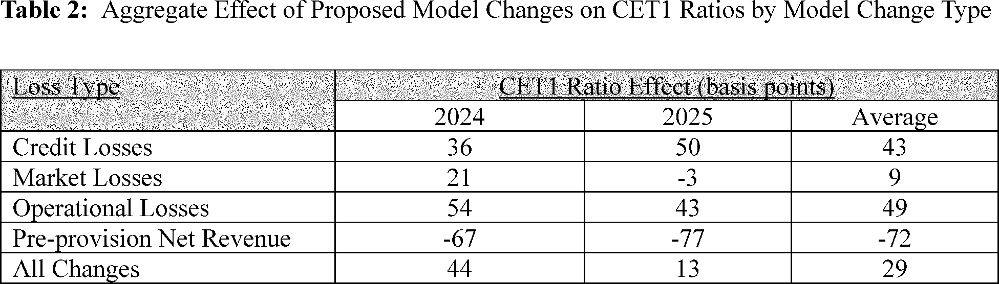
Table 3 below provides a separate analysis of estimates of stress losses across firm types that are subject to the stress capital buffer requirement. The analysis shows the reduction in hypothetical stress losses is concentrated at larger firms.

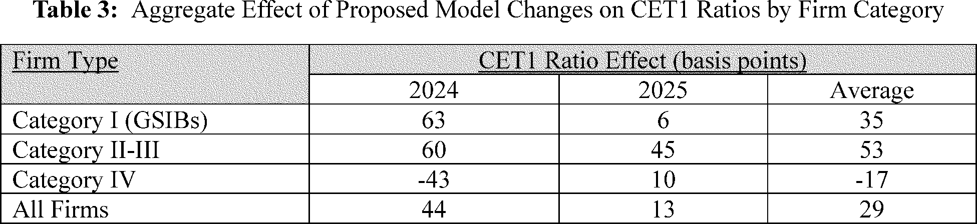
IX. Proposed Changes to the Scenario Design Policy Statement

The Board is also proposing to make several changes to the Scenario Design Policy Statement. While many of these proposed changes are technical in nature, this section identifies substantive changes and requests comment on those proposed changes.

Question 33: The Board invites comment on all aspects of the technical and substantive proposed revisions to the Scenario Design Policy Statement. What are the advantages and disadvantages of these proposed changes? What would be the advantages and disadvantages if the Board were to consider describing the Board's expectations for additional components of the scenario design framework?

A. Changes to the Background and Overview and Scope Sections

The Board is proposing to make limited changes to the first two sections of the Scenario Design Policy Statement, which address background and overview and scope topics, respectively. In the background section, the Board would clarify that the stress tests primarily focus on credit risk, operational risk, and market risk. The inclusion of operational risk in this list helps clarify the Board's continued focus on designing a supervisory tool that makes a valuable forward-looking assessment of large financial companies' capital adequacy under hypothetical economic and financial market conditions. The Board would also clarify that it expects to provide only two different sets of macroeconomic scenarios for both the supervisory and company-run stress tests. These two sets of macroeconomic scenarios are the baseline and severely adverse scenario. This change would clarify the quantity of macroeconomic scenarios the Board expects to provide, consistent with the removal of a separate adverse scenario.^[86]

In the overview and scope section, the Board would make conforming edits to the description of the organization of the Scenario Design Policy Statement to reflect the changes discussed earlier in this proposal.

Question 34: What additional changes, if any, should the Board consider making to these sections, and why? What would be the advantages and disadvantages of providing more than two scenarios? What are the ( printed page 51877) advantages and disadvantages of the Board's continued focus on credit, operational, and market risk?

B. Changes to the Content of the Stress Test Scenarios Section

The Board is proposing to make two general changes to this section, which describes the Board's expectations for the content of the published stress test scenarios.

First, as described below, this section would be amended to clarify that the Board expects to generally publish two different macroeconomic scenarios: the baseline and severely adverse scenarios. This section would also be revised to clarify that the Board expects to invite comment on severely adverse scenarios.

Second, as described in Section IX.H of this Supplementary Information, the Board is proposing to make certain changes related to the global market shock component. See Section IX.H of this Supplementary Information for a discussion of those changes.

Question 35: What additional changes, if any, should the Board consider making to these sections, and why?

C. Approach for Formulating Macroeconomic Assumptions in the Baseline Scenario

The Board is proposing to provide additional details describing the process by which the Board would set the paths of the variables in the baseline and severely adverse scenarios. In particular, the amendments reflect that the Board would post on the Board's website a description of the macroeconomic model utilized to support the construction of the baseline and severely adverse scenarios in the annual stress test. By posting a description of this model (the “macroeconomic model for stress testing”) on the Board's website, the Board expects to improve the transparency, public accountability, and predictability around the Board's scenario design framework, particularly with respect to the baseline scenario and certain variables in the severely adverse scenario. The Board recognizes that, while these enhancements are consistent with the Board's goal of increased transparency in the supervisory stress test, they may constrain the design of the scenario paths for some variables to follow those prescribed by the macroeconomic model for stress testing. Nevertheless, the Board expects that other aspects of the proposed changes to the Scenario Design Policy Statement will preserve sufficient flexibility to allow the Board to adjust the severity of the annual scenario based on relevant indicators of economic and financial conditions and other emergent procyclical factors. Importantly, the Board uses these models to generate paths for the scenario variables only. These models are used solely for stress testing purposes and the output is not a forecast of the Board.

Question 36: What are the advantages and disadvantages of adopting a macroeconomic model for stress testing to guide the selection of certain variables in the baseline and severely adverse scenarios?

Question 37: What additional changes, if any, should the Board consider making to this section, and why?

D. Scenario Narrative: Refinement to the Recession Approach

A number of considerations contribute to the Board's formulation of the severely adverse scenario. As a starting point, the basic approach adopted by the Board is the recession approach— the notion that the Board will construct a scenario informed by the historical paths of macroeconomic and financial market variables across post-war U.S. recessions. However, different recessions have differed in important respects, and a simple recreation of a given episode or an average over all recessions would fail to reproduce important potential stressors to firms' balance sheets. Hence, in applying the recession approach, the Board develops a specific narrative characterizing the hypothetical recession represented by the scenario to help inform the specific paths for scenario variables. This narrative combined with data are then modified to account for the Board's stress testing principle of conservatism alongside other considerations offered by the literature on stress testing including a goal to develop sufficient severity and credibility of the scenarios, and a goal to not add sources of procyclicality to the financial system, as described below.^[87] This section gives an overview of these considerations and other details, providing a common structure for the discussion outlined in the guides for individual variables under this framework, in Section IX.G of this Supplementary Information.

The Recession Approach

The Board intends to continue to use a recession approach to develop the severely adverse scenario. Under the recession approach, the Board expects to specify the future paths of variables to reflect conditions that characterize post-war U.S. recessions, generating either a typical or specific recreation of a post-war U.S. recession. The Board chose this approach in developing past scenarios, and in the Scenario Design Policy Statement, because it has observed that the conditions that typically occur in recessions—such as increasing unemployment, declining asset prices, and contracting loan demand—can put significant stress on firms' balance sheets. This stress can occur through a variety of channels, including higher loss provisions due to increased delinquencies and defaults, losses on trading positions through sharp moves in market prices, and lower bank income through reduced loan originations. For these reasons, the Board expects that the paths of economic and financial variables in the severely adverse scenario should, at a minimum, resemble the paths of those variables observed during a recession. The guide for each variable in this framework reviews the movements of that variable across past recessions and bases the formulation of its scenario path on that analysis. While the recession approach provides a starting point for the formulation of the scenario, recessions are not all the same. The length and depth of recessions differ, as do the parts of the economy and financial markets that are most affected, so the Board must include other considerations in its scenario design.

The Scenario Narrative

Because recessions have differed in cause, character, and consequence—from oil price shocks and housing slumps to asset-price busts and pandemics, from short to long, and from mild to moderate to severe—the Board augments the basic recession approach with an annual scenario narrative. The annual scenario narrative provides qualitative direction on how the Board builds that year's severely adverse scenario.

While some specifics of the narrative may be adjusted on a year-to-year basis to reflect developments in the macroeconomic and financial environment, the overall narrative motivating scenario design will be that of a sharp recession triggered by an adverse shock to financial markets. Under the proposal, the Board expects that the macroeconomic scenario used in the Board's annual supervisory severely adverse scenario will begin with a sudden and significant increase in uncertainty and associated rapid deterioration in risk appetite that cause a spike in financial market volatility and a sharp decline in many U.S. and ( printed page 51878) foreign financial assets. The resulting turmoil would disrupt funding markets and lead to widespread deleveraging, including forced sales of illiquid assets at fire sale prices by a range of financial firms and some temporary breakdowns in the typical correlations between financial asset prices. (Such sharp changes in financial conditions have been observed previously in response to the outbreak of COVID-19 or regional wars, the failure or distress of a large financial institution, or sudden shifts in the economic policies in advanced economies.)

Under the Board's recession approach, the Board expects that, although financial market functioning returns to normal within a few months of the initial shock, uncertainty remains high and risk appetite remains low for an extended period. The sustained flight to quality would be expected to push down risk-free interest rates but keep credit conditions tight and financial asset prices depressed for several quarters. The market dysfunction would cause a contraction in the supply of credit from other types of financial intermediaries that would create demands on banks to provide substantial liquidity to existing customers with formal credit lines. Banks would also make ad hoc decisions to support customers without formal arrangements when doing so could lead to lower losses on their existing loans.^[88] This shift in demand for credit toward banks from other financial intermediaries would lead to banks' balance sheets remaining constant even as overall credit demand declines.^[89] This feature of the scenario is supported by the stress testing principle of conservatism.^[90] To that end, maintaining higher capital requirements during periods of economic expansion ensures that stress tested firms employ sufficient capital to absorb losses and support the economy during a downturn.

In the scenario, the news from financial markets would cause near-immediate decisions by consumers to curtail spending and by businesses to cut payroll and cancel planned investments, leading to a demand-driven contraction in economic activity putting downward pressure on inflation. The initial disruption to spending and employment along with tightening credit conditions would trigger a negative feedback loop that results in further declines in payrolls, investment, and spending in subsequent quarters. With businesses shrinking or failing in the scenario, demand for commercial real estate would decrease significantly relative to supply, leading to large declines in commercial property prices. Meanwhile, rising household financial distress would lead to increased supply of homes for sale and reduced household formation, which would depress residential real estate markets.

The financial market dysfunction and deepening recession in the United States would spill over to its major trading partners, including the euro area, United Kingdom, Japan, and Developing Asia. Those areas would experience declines in economic activity commensurate with the global slowdown running from 2008 to 2010. Consistent with existing stress testing principles, this scenario assumes that permanent government stabilization programs ( e.g., unemployment insurance) and monetary policy in the United States and elsewhere would function normally, but that there would be no extraordinary measures taken by fiscal or financial authorities to support the economy or financial markets during this time. The specific implications of this narrative for scenario variables are detailed in each guide, but the narrative interacts importantly with the recession approach: financial recessions often exhibit different properties than other recessions, as they are often steeper, deeper, and more drawn-out than typical, non-financial recessions.^[91] Adopting this scenario narrative reflects a principle of conservatism, and is in line with recommendations from the stress testing literature, as discussed in Section IX.F of this Supplementary Information.

Question 38: The Board invites comment on all aspects of how the Board designs the scenario narrative in the annual stress test. What are the advantages and disadvantages of adopting this financial recession approach? What other approaches, if any, should the Board consider adopting, and why? What adjustments, if any, to the financial recession approach should the Board consider adopting, and why?

Adding Salient Risks to the Severely Adverse Scenario

Consistent with the Scenario Design Policy Statement, under this proposal, the Board expects that the severely adverse scenario would be developed to reflect the current level of vulnerabilities or risks to the banking sector that are apparent in relevant indicators of economic and financial conditions. The Board anticipates that the proposed guides for certain scenario variables described below provide an appropriate range of values to design the severely adverse scenario in most years. The waxing and waning of relevant indicators of economic and financial conditions will inform the Board's decisions about where to set the value of those parameters within those ranges for each variable.

The Board continues to expect that there will be some important instances when it will be appropriate to augment the recession approach with salient risks and to set variables values inside of, and in some cases, outside of the ranges and values provided in the guides in the Scenario Design Policy Statement. As a result, each year, the Board will consider particular risks to the financial system and to the domestic and international macroeconomic outlook identified by its economists, bank supervisors, and financial market experts. The Board, using its internal analysis and supervisory information and in consultation with the Federal Deposit Insurance Corporation and the Office of the Comptroller of the Currency, will then determine whether any of those risks appear significantly more elevated than usual or, conversely, whether risks are unusually low at a particular time, such that they cannot be appropriately reflected by choosing values within the ranges of the proposed guides. In those cases, which it expects to be infrequent, the Board will make appropriate adjustments to the paths of specific economic variables. These adjustments will not always be reflected in the general severity of the recession and, thus, all macroeconomic variables; rather, the adjustments will sometimes apply to a subset of variables to reflect co-movements in these variables that are historically less typical.

To assist the public in assessing the use of salient risks in the scenario, the Board considered the following examples. A stress test initiated in a ( printed page 51879) period of unusually high uncertainty and rapid deterioration in economic and financial conditions, such as the first quarter of 2009 or the first quarter of 2020, likely would prove challenging for the ranges in this proposed framework. In each case, the prevailing conditions made it plausible that key variables would settle beyond the range of their previous peak or trough values, on which the guides for the variables in the severely adverse scenario are calibrated. Although the unemployment guide remained flexible enough to respond to the spike in the unemployment rate to nearly 15 percent during the first months of the COVID-19-related business closures in 2020, the paths of other variables may have needed to be adjusted more severely if the economy had not recovered as quickly as it did.

As another example, the Board may become increasingly concerned about vulnerabilities related to a particular asset class that was experiencing rapid and persistent price increases supported by increasingly leveraged investors. Those circumstances existed in the housing market in the early 2000s and may have tested the credibility of a guide framework based solely on past performance of home prices, given that up until then, the price index for homes the Board uses for stress testing had rarely experienced a decline.^[92]

Sometimes, the salient risk may arise within an asset class. The Board most recently incorporated this type of salient risk in the 2024 stress test scenario. That year, the Board noted unusually high vulnerabilities in types of commercial properties that could be most at risk for a sustained drop in income and asset values due to the prevalence of remote work.^[93]

The Board is proposing two changes to its consideration of salient risks in the severely adverse scenario. First, the Board would remove paragraph 4.2.4(d) from the Scenario Design Policy Statement. Removing this paragraph could help improve the transparency of the scenario design process by limiting the Board's expectations for considering risks of uncertain significance. While this approach would reduce the Board's ability to test for emerging and untested risks in the financial system through the severely adverse scenario, the Board expects that the remaining components of the Board's supervisory stress test should be sufficient to establish a credible severely adverse scenario.

Second, where the Board does consider salient risks in designing the severely adverse scenario, the Board will endeavor to disclose and explain the Board's reasoning in the Board's publication of the annual stress test scenarios, and subsequently adjust those aspects of the scenario, if necessary, in response to those comments.

Question 39: What are the advantages and disadvantages of the Board's approach to considering salient risks? What additional or alternative approaches, if any, should the Board consider for the consideration of salient risks? What additional or alternative circumstances should the Board take into account when evaluating whether to consider salient risks, if any?

E. Changes to Construction of Certain Variables in the Severely Adverse Scenario

As noted above, the Board finalized changes to the Scenario Design Policy Statement in 2019 that established a guide that it would use in setting the size of the maximum change in the unemployment rate and the timing of its peak. The Scenario Design Policy Statement also introduced a guide to govern the size of the maximum decline in house prices in the severely adverse scenario. This proposal maintains those features of the guides for those two variables, introduces guides that will be used to set the changes in the values, and the timing of those changes, for more variables in the severely adverse scenario, and provides additional context for the path of each variable before it reaches the maximum change. In addition, the Board is separately disclosing a specific macroeconomic model that it proposes to use to translate the paths of certain variables that are set using the proposed guides into internally consistent projections for the remaining variables, such as the 3-month Treasury bill rate, GDP, Disposable Personal Income (DPI), and inflation.

In addition to updating existing guides for the unemployment rate and house prices, the Board is proposing to establish a guide for each of the following variables: equity prices; the VIX index; 5-year Treasury yields; 10-year Treasury yields; BBB corporate bond yields; mortgage rates; commercial real estate prices; and certain international scenario values. These include all but one of the remaining financial market variables typically included in the domestic severely adverse scenario disclosure each year (the exception being the 3-month Treasury bill rate, as discussed below).

The Board uses guides to inform its determination of the behavior of these financial market variables in the severely adverse scenario, rather than model predictions, for several reasons. Although the parameters of the guides are calibrated based on an analysis of historical changes in those variables during recessions and the resulting set of scenario paths typically would be consistent with historical co-movements in those variables, using explicit forward-looking models of these variables to determine scenario paths would be inconsistent with several stress testing principles, such as simplicity and transparency, as described below.

Under a model-driven approach to determine the paths of these variables, each model would require the Board to identify, design, test, explain, and publish additional assumptions, variables, formulas, and parameters that would drive the results of the model. Models of financial market variables can be particularly unreliable during periods of severe stress like the environment envisioned by the hypothetical severely adverse scenario.^[94] Thus, the model-driven approach to determining these variables would contrast with the stress testing principle of using simpler and more transparent approaches, where appropriate.

The Board believes that the guide-based approach also better achieves the stress testing principle of using a stable process that is reliably able to capture the impact of economic stress. These simple, transparent guides also will allow the Board to use its judgment at times when it is necessary to account for conditions that are plausible even if they have not been observed previously, consistent with the stress testing principle of conservatism. Finally, the guides better preserve the Board's ability to adjust the severity of the stress test to avoid adding to procyclical forces, when doing so is appropriate and consistent with fostering financial stability. The Board's judgment about the appropriateness of the annual stress test scenarios will reflect changes in the specific risks or vulnerabilities that the Board, in consultation with the other federal banking agencies, determines should be considered in the annual stress tests.^[95]

( printed page 51880)

The paths for the remaining variables in the domestic scenario—GDP, DPI, inflation, and the 3-month Treasury rate—will be informed by the Board's macroeconomic model for stress testing.^[96] In contrast to the guide-based approach described above for certain variables, the Board uses a model-driven approach for these remaining variables because they are particularly suited to model projections that are simple to produce and explain. As explained in the model documentation available on the Board's website, that model uses a set of well-studied longer-run economic relationships that have proven to be useful in a variety of economic conditions and modeling frameworks. These include Okun's Law, a Phillips Curve, and an inertial Taylor Rule.^[97] The Board acknowledges that increasing the predictability of the paths of scenario variables in this way could reduce the dynamism of the stress test or incent firms to optimize their portfolios in ways that reduce capital requirements, perhaps without a commensurate reduction in risk. However, the guides and the model are constructed to remain flexible enough to ensure that the Board can adjust the severely adverse scenario to capture emerging risks and changes in the level of systemic risk since the previous stress test in a timely fashion. This flexibility includes the ability to increase scenario severity when systemic risks may have built up during robust economic expansions or periods when risk appetite is high or to avoid adding sources of procyclicality through the stress test. The proposal continues to ensure that the scenarios maintain a minimum severity level, even when economic and financial conditions are strained. Setting a floor for the severity of the scenario is appropriate because risks that built up during an economic expansion can persist at financial intermediaries during downturns and because firms that are under stress sometimes take imprudent risks that they believe will facilitate recovery.^[98]

The Board also considered that employing the guides or the macroeconomic model for stress testing sometimes may reduce the severity of some aspects of the scenario relative to what the currently less-constrained scenario design process would achieve, and in other cases it may result in higher severity for some aspects of the scenario than might otherwise be the case. The flexibility in the guides should be sufficient for the Board to account for those eventualities by choosing offsetting values across multiple guides that create the appropriate overall severity of the scenario.

Question 40: What are the advantages and disadvantages of using guides and the macroeconomic model for stress testing to guide the setting of scenario variables in the severely adverse scenario? What, if any, alternatives to using a macroeconomic model to set the projection paths of other variables should the Board consider?

F. Scenario Design Principles Derived from Stress Testing Literature: Severity, Credibility, and Procyclicality

In designing the guides for the construction of the severely adverse scenario presented in this framework, the Board is informed by the stress testing literature, which provides certain principles for scenario design,^[99] which are also reflected in the Board's Stress Testing Policy Statement.^[100] First, the literature emphasizes the need for adequately severe scenarios, even when the economy and financial system are in a stressed condition—complementing the Board's principle of conservatism.^[101] Second, the literature offers insights on how historical data should inform the design of an adequately severe scenario, augmenting the Board's recession approach. Third, the literature highlights the need for stress tests to avoid adding to other sources of procyclicality in the financial system. In explaining the paths for variables in the severely adverse scenario, the guides provide specific applications of these principles, while this introduction provides an overview of their general meaning and rationale.

The first principle derived from the literature concerns the need for sufficiently severe scenarios. Plainly, insufficient stress test severity can lead to adverse outcomes. Inadequately assessed risks lead to an underassessment of the associated credit losses and capital needs—the basic source of failures of many financial institutions during the 2007-2009 financial crisis which the Board's stress tests are meant to avoid. Frame et al. (2015) provide an in-depth analysis of how the assessment of risks (or stress test) conducted by the Office of the Federal Housing Enterprise Oversight (OFHEO) actually contributed to the failures of the Federal National Mortgage Association (Fannie Mae) and the Federal Home Loan Mortgage Corporation (Freddie Mac).^[102] Importantly, stress tests must be adequately severe both in good times and in bad.

In the context of stress testing during crises, in particular, there are additional arguments against insufficient stress test severity. Schuermann (2014) and Judge (2022) argue that insufficiently severe stress test scenarios can erode credibility and trust and impede timely and adequate policy responses to ongoing crisis developments, thereby exacerbating a downturn.^[103] Bernanke (2013) also highlights that stress tests in times of crisis should provide anxious investors with credible information about prospective losses.^[104] This literature points to the importance of sufficiently severe scenarios for the health of the financial system, including by maintaining credibility with the public and financial markets.

Further evidence for the importance of sufficiently stressful scenarios to maintaining public credibility comes from past U.S. stress tests. For example, the rapid deterioration in the U.S. economy in early 2009 led to realized unemployment rates that approached the peak of the unemployment rate path in the severely adverse scenario used for the Supervisory Capital Assessment Program (SCAP) in 2009.^[105] In fact, the scenario peak for the unemployment rate hypothesized would reach only 8.9 percent at the end of 2009, but as of ( printed page 51881) March 2009 the unemployment rate measured 8.5 percent and ultimately the unemployment rate peaked at 10 percent in October of 2009.^[106] Because the results of the SCAP determined the amount of capital that firms needed to raise in financial markets or through the Treasury's Capital Assistance Program, a scenario that turned out to be insufficiently severe could have left some firms undercapitalized and failed to achieve the goal of stabilizing the financial system.^[107]

This example helps demonstrate the importance of the principle of severity when considering historical data and current conditions in the construction of an adequately severe scenario. While unemployment rates are discussed at length in the unemployment guide below, the maximum level of 8.9 percent specified in the 2009 SCAP, at the time, was well beyond the level reached in most post-war recessions. At the time the scenario was issued, a projected increase to 8.9 percent was thus very severe compared to outcomes over the past quarter century, but nonetheless proved lower than the actual realized peak in 2009.

That experience reinforces the need for the framework to support variable paths that exceed levels observed in the historical data. Choosing a historical scenario has a price—“it does not test for anything new.” ^[108] While the recession approach dictates that variable movements follow historical recessions, when current conditions are already extreme, a credible scenario may replicate historical recessions in terms of the size of movements previously observed, leading to levels of variables that may exceed historical levels. Several of the guides in this framework allow, at times, for variables to exceed their historical range, either in levels or in changes, in order to maintain adequate severity.

Ultimately, no single scenario can account for all potential contingencies. Therefore, the severely adverse scenario used in the Board's annual stress test must be sufficiently severe to ensure that banks will be resilient to a range of alternative and plausible scenarios that could generate net losses that are of similar magnitudes.^[109]

At the same time, the Board recognizes that the severity of the annual stress tests potentially can have unintended effects on firms' operations. For instance, the academic literature finds that stress tests improve financial stability by reducing riskier bank lending.^[110] Ensuring that firms are appropriately capitalized for the risks they are taking is a goal of stress testing; however, if those effects are not well aligned with the true riskiness of a particular type of loan, then stress tests could unintentionally reduce banks' credit supply. For instance, some evidence exists that counties in which stress tested banks had high market share may have experienced a lower supply of credit to small and young businesses, which are generally considered riskier than established businesses but can generate a disproportionate share of growth in employment and income.^[111] However, other research concludes that businesses largely offset the reduction in loans from banks that participate in the stress tests with other sources of credit. Those sources include loans from smaller banks not in the stress tests,^[112] debt issuance in capital markets, or loans from nonbank financial institutions.^[113] Moreover, these potential unintended effects on credit supply by stress tested firms must be weighed against the benefits, discussed above, that more credible stress tests bring to the economy and the financial system. By ensuring that firms have sufficient quantity and quality of loss-absorbing capital to cover the risks that they are taking, the stress tests ensure the resilience and stability of the banking sector even in circumstances when stresses take unexpected forms.

The balance of those advantages and disadvantages of scenario severity can change over time. Losses at financial institutions are more likely to arise when the economy slows. Profits are more robust during periods of economic growth, in turn increasing resources available to cover future losses. In other words, capital is naturally procyclical, having an underlying tendency towards a positive correlation with financial conditions. Moreover, when underlying conditions are favorable and firm losses are low, firms sometimes project forward an expectation for low losses, paving the way to take more risk.^[114] Conversely, when conditions are bad, firms may overcompensate and restrict credit even to otherwise creditworthy borrowers, exacerbating the downturn. Thus, firms' behavior may amplify underlying procyclicality.

Stress tests could, through different designs, either amplify or mitigate this procyclicality. If stress tests are always more severe in bad times, despite an expectation that conditions could soon improve, then this severity would add undue stress to the financial system, reducing financial intermediation with negative implications for the macroeconomy. That said, the purpose of the stress test scenarios is not to serve as an explicit countercyclical offset to the financial system, but rather to ensure that the firms are properly capitalized to withstand severe economic and financial conditions. Hence, the Board adopts a middle path, seeking to specify the severely adverse scenario to avoid adding sources of procyclicality to the financial system, neither explicitly mitigating any existing procyclical tendencies nor magnifying them. Indeed, Kohn and Liang (2019) argue that the ability to adjust elements that potentially add procyclicality can be a major benefit of stress tests as “banks with forward-looking, less-procyclical capital buffers will not pull back as much when a downturn occurs.” ^[115]

In summary, in formulating the guides presented in this framework, the Board embraces three principles suggested by the literature: the importance of severity, the importance of credibility, ( printed page 51882) and the importance of not adding to procyclicality.

Stress Testing Literature and the Principle of Flexibility

When considering these principles in light of the recession approach and the scenario narrative, the Board identified the importance of maintaining flexibility in the guides. While the Board intends to increase the transparency, public accountability, and predictability of stress tests through this proposal, these goals should not come at the expense of the overall effectiveness of the Board's stress tests.

For instance, predictability and transparency could be achieved with a completely specified, entirely formulaic scenario that leaves no flexibility. However, simple, fixed guides may not achieve at least one of the goals of severity, credibility, or not adding to procyclicality. A guide that always increased unemployment to a fixed level, say 10 percent, may not be credible or severe were the unemployment rate already at or close to that level. A guide that always increased unemployment by a fixed amount, say 4 percent, could add to procyclicality by implying lower losses when unemployment was low in good times and higher losses when unemployment was high in bad times. More sophisticated formulations might improve on simple rules by accounting for the factors affecting firms' balance sheets and overall economic and financial conditions. For many types of economic indicators used in the Board's scenario framework, however, a fixed rule for the design of a scenario variable that satisfied the principles related to procyclicality and severity laid out above could require a complex structure that would violate the Board's principle of simplicity.^[116]

A lack of simplicity is not, however, the only concern with a framework that eliminates flexibility. Unexpected shocks occur, like oil embargoes, national house price collapses, and pandemics. Moreover, the implications of these shocks are often not readily captured in concurrent data, especially their future effects on the economy and financial stability in the United States, and so on firms' future financial condition. Maintaining a degree of flexibility would allow the scenarios to adapt to evolving conditions while adhering to the principles outlined above.

In specifying the guides in this framework, the Board seeks to maintain flexibility by specifying ranges for the peak or trough value, the timing of that value, or the speed of adjustment for many of the variables. The amount of flexibility in the guides, as measured by the size of ranges specified, is calibrated to be as narrow as possible while adhering to the principles laid out above and is based on research and analysis of the behavior of those variables during past recessions, consistent with the recession approach, or periods of stress in financial markets. In addition to suggesting typical ranges within which scenarios will vary, the Board seeks to provide explanations of how the guide flexibility would be applied in different economic and financial conditions.

Generally speaking, the Board would design a more severe path for the scenario variables when it judged the level of systemic risks to be high, and a less severe path for the scenario variables when it judged systemic risks to be low. In some cases, the level of systemic risk can be tied to the level of specific indicators. For instance, when the unemployment rate is very high, the level of risk aversion also tends to be high, and that causes firms to reduce risk across their various business lines. In other cases, the Board would consider overall assessments by economists, supervisors, and financial market experts to assess the level of systemic risks, which typically incorporate many of the specific indicators mentioned in the discussions of individual guides below, when it is difficult to do so using individual or small sets of scenario variables.^[117]

Therefore, the Board expects that it may choose to have similar severities for variable values in an annual scenario for those variables where the Board retains discretion within established ranges of the proposed guides. This expectation reflects the Board's consistent view that annual scenarios are not forecasts of potential future outcomes in the baseline or in a hypothetical stress environment. Establishing variable values with similar severity levels enhances the transparency and predictability of the annual scenarios, and reflects an expectation that these variables are likely to experience stress concurrently in a hypothetical stress scenario. As discussed below, if the Board were to determine that a specific salient risk should be addressed in a particular annual stress test, it would provide a specific assessment of that risk and the rationale for an alternative calibration of the variable's severity in the scenario disclosure for comment.

While flexibility allows scenarios to adapt to fast-evolving conditions, the guides in this framework are based on long-lasting structural features of the economy. Macroeconomic history, however, features many examples where new data have contradicted long-held beliefs about underlying structural relationships. Also, the financial system is constantly evolving, presenting new risks and vulnerabilities. The relatively narrow ranges in the guides may not always allow for a fulsome response by the scenarios to significant developments. Therefore, the Board also sets out expectations for circumstances that could require additional flexibility in setting the specifications of the variables in the stress tests, so that the public can anticipate where the Board could adopt a specification that differs from those identified in the guides in this proposal. For instance, if events occur that alter the historical severity of a given variable, the Board could incorporate that data in its evaluation of the appropriate path for a given variable in annual scenarios that occur following such an event. The Board continuously monitors the macroeconomy and the financial system. If ongoing developments warrant, the Board may revisit this framework and adjust guides.

Finally, the increased predictability and transparency of the scenario as specified in this framework may allow firms to adjust their portfolios to reduce capital requirements, perhaps without a commensurate reduction in risk. While the Board acknowledges this possibility, the Board expects that the principle of severity embraced in this framework will produce scenarios that adequately test such risks. Flexibility is maintained to allow scenarios to adapt to evolving conditions, not to reduce predictability and transparency. Indeed, the ranges of flexibility specified, especially when considered alongside the guidance offered regarding the conditions under which that flexibility might be employed, result in highly transparent and predictable scenario paths. Overall, the Board finds that the degree of flexibility and the goals of transparency and predictability are well balanced by this proposal, given the other requirements for designing effective and credible stress tests.

Summary of Scenario Design Principles

In formulating the guides presented in this framework, the Board is proposing to continue to use a recession approach, ( printed page 51883) where the severely adverse scenario reflects conditions that characterize post-war U.S. recessions. To implement this approach, the Board adopts a specific scenario narrative in which a severe shock to financial markets propagates through the economy and results in a severe, prolonged recession most similar to that of the 2007-2009 financial crisis. The Board provides a qualitative description of the scenario informing the hypothetical recession that the scenario reflects. In choosing specific scenario paths, the Board recognizes a need for the scenario to be adequately severe and credible, and to avoid adding to procyclicality.^[118] Finally, in this pursuit, the guides maintain a degree of flexibility to adapt to evolving economic and financial conditions. The Board continues to expect that there will be some important instances when it will be appropriate to augment the recession approach with salient risks and to set variables' values inside of, and in some cases, outside of the ranges and values provided in the guides in the Scenario Design Policy Statement.

Question 41: What are the advantages and disadvantages of selecting the scenario design principles described in this section? Are there other principles that the Board should weigh along with these principles? Should the Board develop guidance for how it would weigh these principles in selecting values in annual scenario narratives?

Question 42: What considerations should the Board evaluate when determining whether to set a given scenario variable independently of other variables in the annual scenario, or at similar levels of severity across multiple variables?

Common Components of Scenario Path Guides

The guides in this framework set out paths for each variable over the 13 quarters in the severely adverse scenario. The stress test requires projections of 13 quarters worth of losses to determine capital ratios at the end of 9 quarters of the scenario, because loss provisions in quarter 9 are affected by firm performance in quarters 10 to 13. To describe these paths, most guides adopt a simple framework involving the following four parameters: the jump-off; the peak or trough; the timing of the peak or trough; and the trajectory from jump-off to peak or trough. The purpose of publishing these components is to increase the transparency and public accountability of the stress test scenario by communicating how the variable would behave throughout the scenario period. In calibrating these parameters, the guides explain their rationale in applying the recession approach along with the scenario narrative and the three principles for scenario design described above. These parameters are described as follows:

Jump-off: Jump-off values are important for informing the overall state of the economy in the scenarios, often affecting the specific levels achieved by the other parameters of the variable guide and informing the exercise of flexibility as specified in the guides. In the scenario, the jump-off value is the value of the variable in the quarter preceding the scenario. For most variables, the jump-off value is easily determined from published data at the time the scenario is released to the public. However, for some variables the jump-off value is not available prior to the date that the Board must finalize the annual scenarios for publication, so an estimate is used; these details are described in the individual guides. A separate issue involves choosing the appropriate historical jump-off date in the Board's analysis underlying the calibration of the guides. In many cases, stresses developed over time and a specific jump-off date or quarter for a particular period of stress may not be clearly identifiable. For instance, the 2007-2009 financial crisis had multiple newsworthy events—the suspension of redemptions from money market mutual funds by BNP Paribas in August 2007, the failure of Bear Stearns in February 2008, and the bankruptcy of Lehman Brothers in September 2008. Therefore, the Board uses a range of quarters around the beginning of an identified recession or period of market stress to determine the jump-off values. The Board determined that using the most extreme value of the variable in the four quarters before, and the first quarter of, the National Bureau of Economic Research (NBER) recession date or documented financial stress event as the starting point for the analysis supporting the calibration of the severity of the guides was most consistent with the Board's stress testing principle of conservatism. Each guide provides further details on selection of relevant reference periods.

Peak or trough: The paths in the guide specify that each variable in the scenario will either increase or decrease from its jump-off value. If it increases, it will reach a maximum or peak value during the scenario. If it decreases, it will reach a minimum or trough value during the scenario. For example, during the scenario, unemployment initially increases to a peak value, while house prices decrease to a trough value. Each guide provides details on how the Board expects to determine the level of this peak or trough and the rationale for this determination. In general, more extreme values are more stressful, and the specific levels of the peak or trough often depend on the jump-off values in line with the principles of severity, credibility, and not adding to procyclicality.

Trajectories from jump-off to peak or trough: This parameter describes the values between the jump-off and peak or trough with a straight line (linear) function, a nonlinear function, or by specifying the proportion of the change from jump-off to peak or trough that will obtain in each of the intervening quarters. Two further notes on trajectories: first, trajectories are frequently described as either frontloaded, meaning that larger changes occur earlier in the trajectory, or backloaded, meaning that larger changes occur later in the trajectory. Depending on the variable, frontloading and backloading affect the overall severity of the scenario by having stressful changes earlier or lasting longer. The individual guides discuss this issue. Second, while several of the guides specify precise mathematical formulas for trajectories, for example linear (straight line) trajectories, rounding conventions—such as rounding to the first decimal place—for the published scenario may result in small differences from the result specified by the underlying formula. These rounding conventions result in small changes to scenario variables that tend not to affect overall severity. Instead, such rounding conventions are meant to help simplify the communication of the scenario to the public.

The Board also considered the appropriate trajectory of variables after they reach the peak or trough and the appropriate end value. This analysis confirmed that the range of end values used in past stress tests are generally supported by historical analysis combined with the stress testing ( printed page 51884) principle of conservatism. The end value describes the value of the variable in the last (13th) quarter of the scenario. In applying the recession approach to calibrating end-values, the Board considers the values of a variable within a 10-15 quarter window after the beginning of the recession or other identified financial stress event, instead of simply taking the value of the variable in the 13th quarter. This range of values allows the Board to better assess outliers or other interactions between the data and the annual scenario narrative than other calibration methods. This flexibility also helps accommodate choices that account for the highly variable lengths of historical recessions. The Board expects that for most variables determined by guides, the recovery trajectories between the peak or trough and end value typically should follow a roughly linear path that proportionally allocates the change across the relevant time remaining to the end of the scenario. A roughly linear recovery reflects a preference for simplicity and transparency. For variables determined by the Board's macroeconomic model for stress testing, the end values and related trajectory from the peak or trough generally will be determined by the model.

Timing of peak or trough: The guides for each variable set out the quarter of the scenario in which the variable path reaches its peak or trough. Generally, these occur earlier for fast moving variables and later for slow moving variables. Depending on the variable, either earlier or later timing may be more stressful, and there may be some flexibility in the timing of the peak or trough.

In developing this framework, the Board considered a number of alternative specifications, both for specific variables and for the overall approach. Some of these alternatives are described in greater detail within the discussion of each proposed guide in Section IX.G of this Supplementary Information.

As described in the Scenario Design Policy Statement, the Board considered alternatives to the recession approach for the overall design of the severely adverse scenario, including a probabilistic approach. The probabilistic approach would construct a baseline forecast from a large-scale macroeconomic model and identify a scenario that would have a specific probabilistic likelihood, given the baseline forecast. The Board believes that, at this time, the recession approach is better suited for developing the severely adverse scenario than a probabilistic approach because it guarantees a recession of some specified severity. In contrast, the probabilistic approach requires the choice of an extreme tail outcome—relative to baseline—to characterize the severely adverse scenario ( e.g., a five percent or a one percent tail outcome). In practice, this choice is difficult as adverse economic outcomes are typically thought of in terms of how variables evolve in an absolute sense rather than how far from the baseline they lie in the probability space. In this sense, a scenario featuring a recession may be somewhat clearer and more straightforward to communicate. Finally, the probabilistic approach relies on estimates of uncertainty around the baseline scenario and such estimates are in practice model-dependent.

The Board also considered two types of alternative specifications for each of the guides. First, the Board considered a more-prescriptive approach, in which the guides set a typical peak or trough value and a specific quarter in which that value would obtain, usually either at the most severe end of the range specified in the proposed guide or at the mid-point of the range. A guide set at the most severe end of the range would be consistent with the principle of conservatism and provide a high degree of transparency and predictability. In contrast, the lack of flexibility in such a guide would reduce the ability of the Board to respond appropriately to risks that are apparent in relevant indicators of economic and financial conditions and could potentially add to procyclical forces during economic booms or stressful periods. A guide benchmarked to the midpoint of the range might not be credible during periods of high vulnerability, while still being too severe when stresses were already present.

Second, the Board considered that guides could have larger ranges for the potential peak or trough values or the timing of the peak or trough than the proposed guides. Larger ranges would increase the Board's ability to capture risks that are apparent in relevant indicators of economic and financial conditions and to adjust to procyclical forces but would be less predictable and transparent. In general, the Board expects the lower end of the range chosen for the proposed guides to represent the least amount of stress that would be deemed credible, while the higher end of the ranges already reflects the most severe plausible realizations of the variable. The proposed ranges for the guides are benchmarked to historical experience while still providing some ability to move beyond the upper or lower end of the historical range if circumstances dictate. In consideration of these factors and the principles discussed above in this section, therefore, the Board expects that the disadvantages from the loss of transparency and predictability from guides with larger ranges generally would be larger than the advantages stemming from more flexibility in the wider ranges of such guides.

In each case, the proposed and some specific examples of alternative guides are both discussed. While the Board views the alternative guides as reasonable, the proposed guides have significant advantages over the considered alternatives. However, the purpose of the alternative guide discussion is to invite comment on a reasonable alternative considered by the Board and to transparently lay out the Board's present decision making in not adopting it.

Question 43: What are the advantages and disadvantages of the alternative guides? Should the Board consider adopting any of the alternative guides? What, if any, other guides should the Board consider in addition to the alternative guides considered?

G. Description of Variable Guides in the Severely Adverse Scenario

Unemployment Rate

The stress test scenarios set out trajectories for several variables, including the unemployment rate of the civilian non-institutional population aged 16 and over (unemployment rate).^[119] As described in the previous sections, the Board intends to use a recession approach to develop the severely adverse scenario. The most common features of recessions are increases in the unemployment rate and contractions in aggregate incomes and economic activity. For this and the following reasons, the Board intends to use the unemployment rate as the primary basis for specifying the severely adverse scenario. First, the unemployment rate is likely the most representative single summary indicator of adverse economic conditions. Second, in comparison to GDP, labor market data have traditionally featured more prominently than GDP in the set of indicators that the NBER reviews to inform its recession dates.^[120] Third and finally, the growth rate of potential output can cause the size of the decline ( printed page 51885) in GDP to vary between recessions. While changes in the unemployment rate can also vary over time due to demographic factors, this seems to have more limited implications over time relative to changes in potential output growth. The unemployment rate used in the severely adverse scenario will reflect an unemployment rate that has been observed in severe post-war U.S. recessions, measuring severity by changes in the unemployment rate and GDP.^[121]

The Board uses a quarterly average of the monthly unemployment rate data in the stress test scenarios. The Board uses a quarterly average of unemployment for several reasons. Unemployment and, importantly, related variables such as disposable income (discussed below) can feature volatility at higher frequencies unrelated to underlying market conditions ( e.g., unexpected weather events or a baseline level of statistical variation in the survey responses); quarterly averages smooth out the volatility that is present at monthly frequencies. Overall, using quarterly averages strikes a balance between being sensitive enough to capture broader economic trends and stable enough to avoid overreaction to short-term fluctuations. The Scenario Design Policy Statement outlines certain information regarding the peak level and timing of the peak level of the unemployment rate for the severely adverse scenario.^[122] This proposed guide conforms with and expands on that statement, providing greater predictability, transparency, and specificity with regards to the trajectory to peak value. The remainder of this section is outlined as follows. An overview of the unemployment guide components is given in Table 4. This is followed by a reiteration of the Scenario Design Policy Statement which describes the peak component of the unemployment rate and its timing. After that, a discussion of the trajectory to peak value is provided.

The purpose of publishing these components is to increase the predictability, public accountability, and transparency of the stress test scenario by communicating how the variable will behave throughout the scenario period.

( printed page 51886)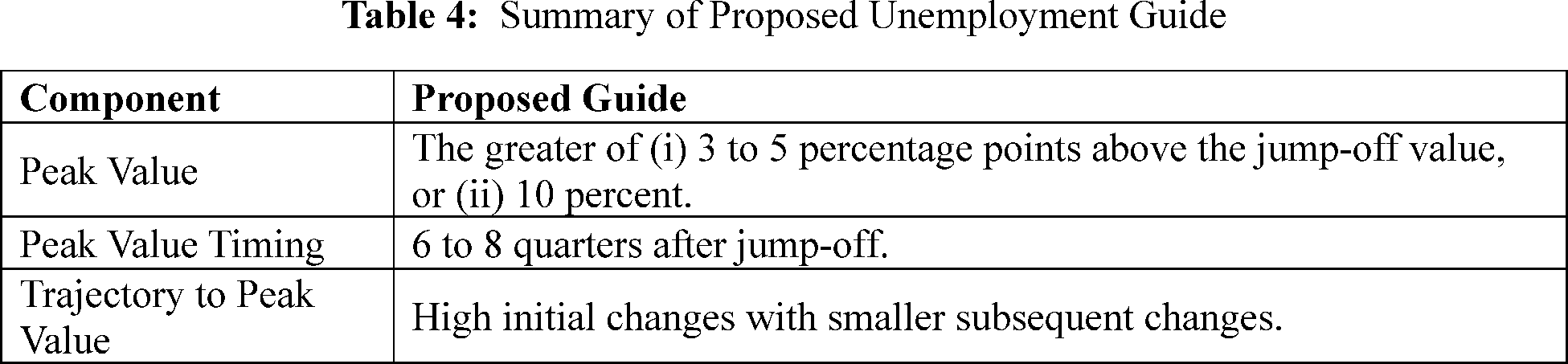

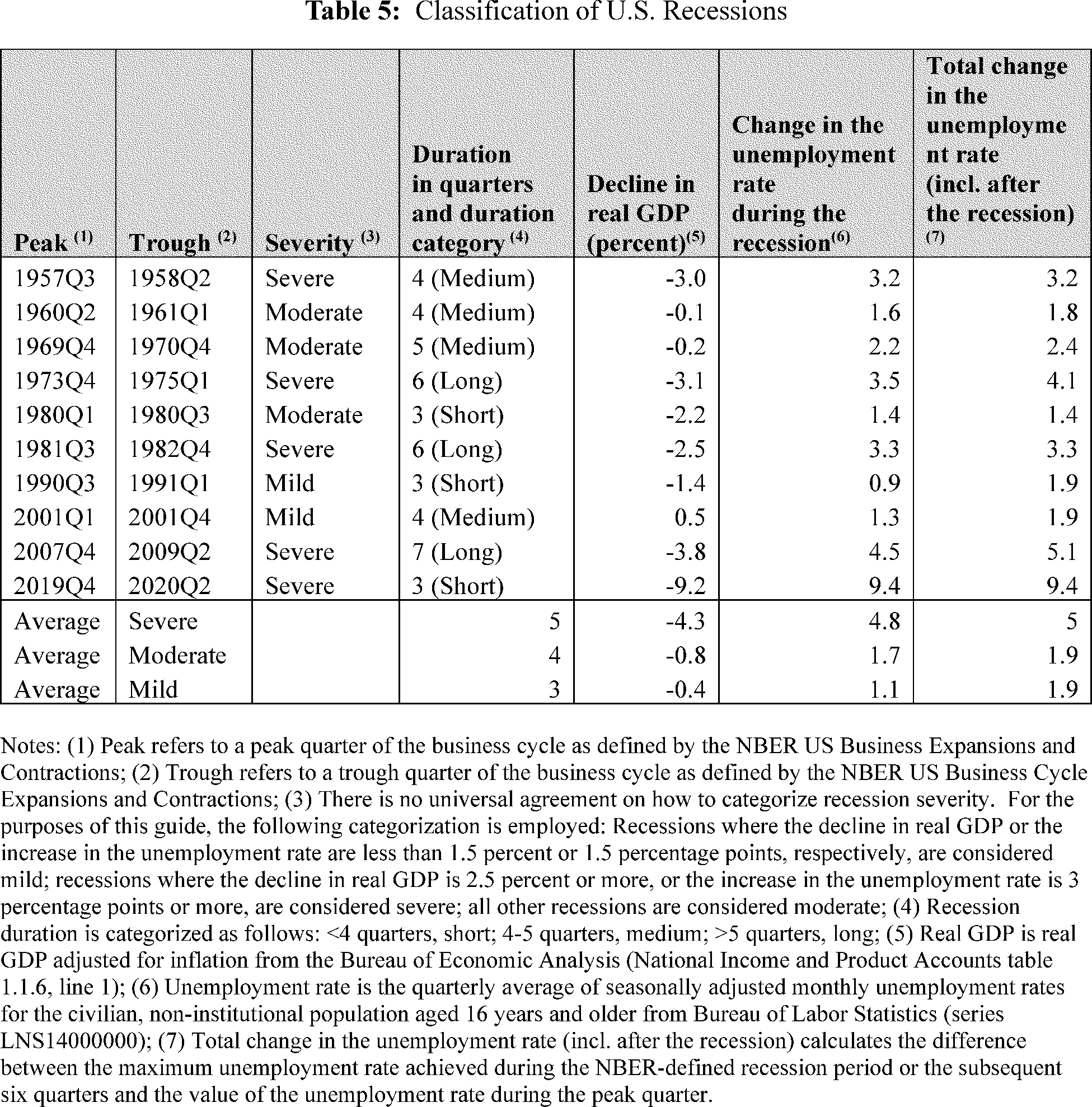
a. Peak Value and Timing of Peak

The Board is proposing to retain the guide established in the Scenario Design Policy Statement, with some additional explanations provided here. The Board anticipates that the severely adverse scenario will feature an unemployment rate that increases between 3 to 5 percentage points from its initial level over the course of 6 to 8 calendar quarters.^[123] The initial level will be set based on the conditions at the time that the scenario is designed. However, if a 3 to 5 percentage point increase in the unemployment rate does not raise the level of the unemployment rate to at least 10 percent—the average level to which it has increased in severe recessions—the path of the unemployment rate in most cases will be specified so as to raise the unemployment rate to at least 10 percent.

This methodology is intended to generate scenarios that feature stressful outcomes but do not add to procyclicality in the financial system and macroeconomy.^[124] When the economy is in the early stages of a recovery, the unemployment rate in a baseline scenario generally trends downward, resulting in a larger difference between the path of the unemployment rate in the severely adverse scenario and the baseline scenario, resulting in a severely adverse scenario that is relatively more intense. Conversely, in a sustained strong expansion—when the unemployment rate may be below the level consistent with full employment—unemployment ( printed page 51887) in a baseline scenario generally trends upward, resulting in a smaller difference between the path of the unemployment rate in the severely adverse scenario and the baseline scenario, resulting in a severely adverse scenario that is relatively less intense. Historically, a 3 to 5 percentage point increase in the unemployment rate is reflective of stressful conditions. As illustrated in Table 5, over the last half-century, the U.S. economy has experienced five severe post-war recessions. In all of these recessions excluding COVID-19, the unemployment rate increased 3 to 5 percentage points, and in the three most recent of these recessions excluding COVID-19, the unemployment rate reached a level between 8 percent and 11 percent.^[125]

Under this method, if the initial unemployment rate were low—as it would be after a sustained long expansion—the unemployment rate in the scenario would increase to a level as high as what has been seen in past severe recessions. However, if the initial unemployment rate were already high—as would be the case in the early stages of a recovery—the unemployment rate would exhibit a change as large as what has been seen in past severe recessions.

The Board expects that the typical increase in the unemployment rate in the severely adverse scenario will be about 4 percentage points. However, as discussed in Section IX.F of this Supplementary Information, the Board expects to calibrate the increase in unemployment based on its views of the status of cyclical systemic risk. More specifically, the Board would be more likely to set the unemployment rate at the higher end of the range if the Board expects that cyclical systemic risks are high (as it would be after a sustained long expansion), and alternatively would be more likely to set the unemployment rate to the lower end of the range if cyclical systemic risks are low (as it would be in the earlier stages of a recovery), provided doing so remained consistent with the goal of ensuring that firms were properly capitalized to withstand severe economic and financial conditions. This may result in a scenario that is slightly more intense than normal if the Board expects that cyclical systemic risks were increasing in a period of robust expansion.^[126]

Conversely, it would also allow the Board to specify a scenario that is slightly less intense than normal in an environment where systemic risks appeared subdued, such as in the early stages of a recovery. This choice would consider that the scenario does not add unduly to remaining stress, thereby exacerbating the initial adverse shock, and it would be particularly appropriate if the Board judges that firms are already taking steps to reduce their risk—for instance, by potentially restricting lending to otherwise qualified borrowers. The Board expects that, in general, it would adopt a change in the unemployment rate of less than 4 percentage points when systemic risks are low or receding. This might be the case when, along with other factors, the unemployment rate at the start of the scenarios is elevated but the labor market is judged to be strengthening and higher-than-usual credit losses stemming from previously elevated unemployment rates were already realized—or are in the process of being realized—and thus removed from firms' balance sheets.^[127] However, even at the lower end of the range of unemployment-rate increases, the scenario would still be expected to feature an increase in the unemployment rate similar to what has been seen in about half of the severe recessions of the past 50 years.

As indicated previously, if a 3 to 5 percentage point increase in the unemployment rate does not raise the level of the unemployment rate to 10 percent—the average level to which it has increased in severe recessions—the path of the unemployment rate will be specified so as to raise the unemployment rate to 10 percent. Setting a floor for the unemployment rate at 10 percent recognizes the fact that not only do cyclical systemic risks build up at financial intermediaries during robust expansions, but also that these risks are easily obscured by a buoyant environment.^[128]

In setting the increase in the unemployment rate, the Board will consider the extent to which analysis by economists, supervisors, and financial market experts finds cyclical systemic risks to be elevated (but difficult to be captured more precisely in one of the scenario's other variables).^[129] In addition, the Board—in light of potential impending shocks to the economy and financial system—expects to also take into consideration the extent to which a scenario of some increased severity might be necessary for the results of the stress test and the associated supervisory actions to sustain public confidence in financial institutions. Some indicators that would inform the Board's decision would be the growth rate of real GDP and its trajectory in recent quarters as well as leading economic indicators, such as equity prices as these measures provide a broader perspective on the state and direction of the economy. Consistent with the Scenario Design Policy Statement, the Board is mindful of sources of procyclicality in the financial system and in designing the severely adverse scenario. While the Board designs the stress test scenarios to promote the proper capitalization of firms, the scenarios are not intended to serve as an explicit countercyclical offset to the financial system.^[130]

Alternative Peak Guide Options

In preparing this proposal, the Board considered a guide that would choose a peak level for unemployment that is 4 percentage points higher than the jump-off value or 10 percent, whichever is higher. This alternative has the advantage of being simpler, more predictable, and more transparent than the guide choice. The Board views this alternative guide to be less desirable as it is less flexible and may end up being inadequately severe. Furthermore, such lack of flexibility could potentially add to scenario procyclicality. For example, in periods with already highly elevated unemployment rates above 7 percent, this alternative could result in unemployment rates of historically high levels at times when economic conditions were already depressed.

Instead, the current guide, specifying the greater of an increase of 3 to 5 percentage points or 10 percent, acknowledges that the Board would be unlikely to consider larger changes in unemployment when its rate is already highly elevated. As discussed in Section IX.F of this Supplementary Information, when the underlying conditions are favorable and firm losses are low, firms may project these tendencies forward, ( printed page 51888) paving the way to take more risk.^[131] Similarly, as discussed previously, the ability to adjust elements that potentially add procyclicality can be a major benefit of stress tests.^[132]

b. Trajectory to Peak

The Board anticipates that the severely adverse scenario would feature a trajectory to the peak unemployment rate that initially increases quickly with slower incremental increases. The trajectory to peak will have a concave parabolic path starting from the value in the economy at the beginning of the scenario and reaching a peak at between 6-8 quarters.^[133] This approach for the trajectory to peak reflects several considerations. First, this trajectory to peak features larger increases in unemployment in the early quarters of the scenario, reflecting a rapid and deep deterioration in labor market conditions, in line with the scenario narrative discussed above and consistent with the principle that the severely adverse scenario be highly stressful as a rapid increase gives firms less time to adapt to changes. Second, this trajectory to peak is consistent with theoretical economic models which often share the feature that the response of unemployment to a shock features initially large increases in unemployment with decreasing incremental changes up to the peak.^[134] Empirically, this general pattern can be seen, for example, in the impulse response function illustrated in the first panel of Figure 2 in the FEDS Note that evaluates empirical regularities in variable co-movement in stress test scenarios.^[135] Third, while all recessions have differences in their specific paths of the unemployment rate, a concave trajectory to peak is broadly consistent with the data from severe recessions. One indicator is to look at second differences, which are the change in changes, an approximation of the acceleration of a variable.^[136] Concave paths have negative second differences. The second differences of the unemployment rate are negative on average for severe recessions, indicating a generally concave path with decreasing changes up to the peak.

Finally, a trajectory with frontloading of increases in the unemployment rate has been a characteristic of all recent severely adverse scenarios, except for the second round of bank stress tests in September 2020.^[137]

House Prices

The stress test scenarios set out trajectories for several variables, including house prices as measured by the Price Index for Owner-Occupied Real Estate (HPI).^[138] The Scenario Design Policy Statement outlined information regarding the formulation of house prices in the severely adverse scenario. This guide conforms with and expands on that statement, providing further information on the data used in the construction of the house price path in the severely adverse scenario, including the timing of the trough value and the trajectory to the trough value.^[139]

Firms subject to the supervisory stress test have a substantial exposure to the residential real estate market.^[140] Given firms' direct exposures, and the broader impact of the housing sector on household balance sheets and the macroeconomy, the Board's methodology for supervisory stress tests incorporates house prices into a number of models.^[141] Moreover, house price build-ups sometimes precede episodes of banking stress, with a notable example being the 2007-2009 financial crisis. By incorporating house prices into macroeconomic scenarios, supervisory stress tests help ensure that firms subject to the stress test are prepared for a range of market outcomes, including periods of large declines in house prices directly affecting loan performance and firms' balance sheets. This helps maintain the overall stability and resilience of the financial system.

The Board uses a quarterly average frequency for this data in the supervisory stress test scenario. Instead of using the monthly frequency at which the underlying data is available, the Board uses a quarterly average of house prices in the stress test scenario for several reasons. House prices and, importantly, related variables such as disposable income (discussed more below) can feature volatility at higher frequencies unrelated to underlying market conditions. For example, extreme weather can affect the demand for home purchases and employment during a particular month, and thus the prices paid in home transactions and income that month, notwithstanding market conditions. Therefore, quarterly averages smooth out month-to-month volatility. Overall, using quarterly averages strikes a balance between being sensitive enough to capture market trends and stable enough to avoid overreaction to short-term fluctuations in prices.

In determining the appropriate level of scenario severity, the Board adheres to the scenario design principles discussed in Section IX.F of this Supplementary Information. While doing so, the Board also strives to avoid introducing additional sources of procyclicality into the financial system. In the context of house prices, these principles are applied in calibrating the key aspects of the guide: the trough value, the timing of the trough value, and the trajectory to trough value. This approach helps ensure that the house price guide aligns with the established stress testing literature while mitigating potential systemic risks for the financial system. This guide description is outlined as follows. An overview of the house prices guide is given in Table 6. This is followed by a reiteration of the Scenario Design Policy Statement which describes the trough value used in the ( printed page 51889) construction of house prices. After that, this guide provides a supplementary discussion of the construction of house prices in the severely adverse scenario, followed by a discussion of the other components of the trajectory of house prices.

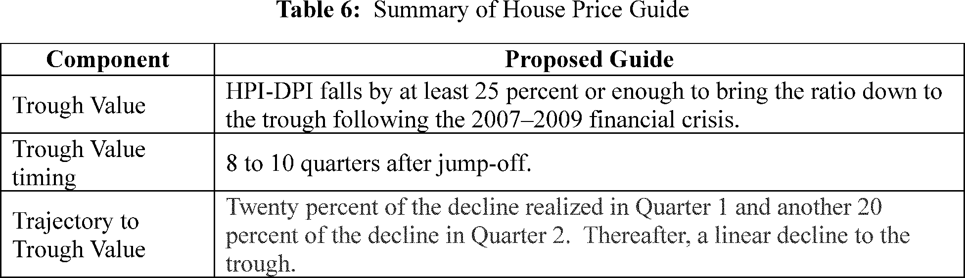
a. Trough Value Component of the Guide

The Board is proposing to retain the guide established in the Scenario Design Policy Statement to inform the trough of house prices in the scenario, with additional explanations provided here. In most circumstances, the Board expects that the ratio of HPI to nominal per capita DPI (HPI-DPI ratio) falls by at least 25 percent or enough to bring the ratio down to the trough reached in the wake of the 2007-2009 financial crisis, which occurred in the first quarter of 2012, whichever is greater.

Data- and Scenario-Based Rationale for the Trough Value

Declining house prices, which are an important source of stress to a firm's balance sheet, are not a steadfast feature of recessions, and the historical relationship of national house prices with the unemployment rate is not strong. Simply adopting their typical path in a severe recession would likely underestimate risks stemming from the housing sector. This can be seen when considering regional housing recessions, which have occurred with greater frequency. Three examples include New England and California in the early 1990s, and Texas in the 1980s. While regional house price indices featured only moderate decreases, the ratios of price to income fell precipitously. Further, in each case, the regional housing recession precipitated a regional banking crisis.¹⁴²

Assessing the procyclicality of house price paths over time is complicated by the fact that house prices—in contrast to the unemployment rate—have historically trended upward over time. Therefore, instead of specifying the path of house prices directly, the Board expects to consider the ratio of the nominal HPI to nominal per capita DPI. The HPI-DPI ratio does not exhibit an upward trend and, as such, provides an alternative way to assess the procyclicality of the scenarios' house price paths. Moreover, the HPI-DPI ratio is a commonly used valuation metric for the housing sector.^[143]

Under most circumstances, the Board expects the decline in the HPI-DPI ratio in the severely adverse scenario to be 25 percent from its starting value or enough to bring the ratio down to its trough during the 2007-2009 financial crisis, whichever is the larger decline. The maximum trough level specified in this guide is motivated by the data, corresponding to the level achieved in the wake of the 2007-2009 financial crisis, which reached a trough in the first quarter of 2012. The minimum decline specified in this guide for the HPI-DPI ratio from its starting value, a 25 percent decline,is motivated by the data as well—such a fall reflects the average peak to trough fall in this ratio across the three national housing recessions identified by the Board, as shown in Table 7.^[144] While the average across housing recessions is heavily influenced by the steep decline in the 2007-2009 financial crisis, similar magnitude falls have occurred with greater frequency when considering the

( printed page 51890)

aforementioned regional housing recessions.^[145]

The minimum decline of 25 percent ensures adequate scenario severity, maintaining the credibility of the stress test while at the same time constraining the trough from becoming unduly contractionary and deviating too far from historically observed levels.^[146] Applying a larger value of a minimum decline ( e.g., the 2007-2009 peak-to-trough fall of more than 40 percent) could result in a trough level that is unjustifiably far away from most historical movements, especially if it were applied during a period in which the HPI-DPI ratio were already at a low level. Alternately, specifying a maximum trough level higher than that experienced during the 2007-2009 financial crisis might not allow the Board to adequately test firms' resilience to potential shocks when home valuations are as elevated as they were in the mid-2000s.

The construction of this part of the house prices guide reflects the goal of avoiding adding sources of procyclicality in the financial system. Accordingly, the severely adverse scenario will feature smaller variable movements when those variables are less extreme, and the severely adverse scenario will feature larger variable movements when those variables are more extreme, generally up to a level at least as extreme as the 2007-2009 financial crisis.

The recession approach provides further justification for the proposed calibration of the severity of the trough of house prices. While national house prices and national unemployment do not exhibit a strong relationship in the data, research shows that unemployment in a household has a large effect on default rates, and that increases in local unemployment are correlated with decreases in local house prices.^[147] Similarly, regional housing recessions often feature increases in regional unemployment.^[148] Hence, the recession approach suggests that a scenario with a high peak level of unemployment should also feature a low nadir in house prices.

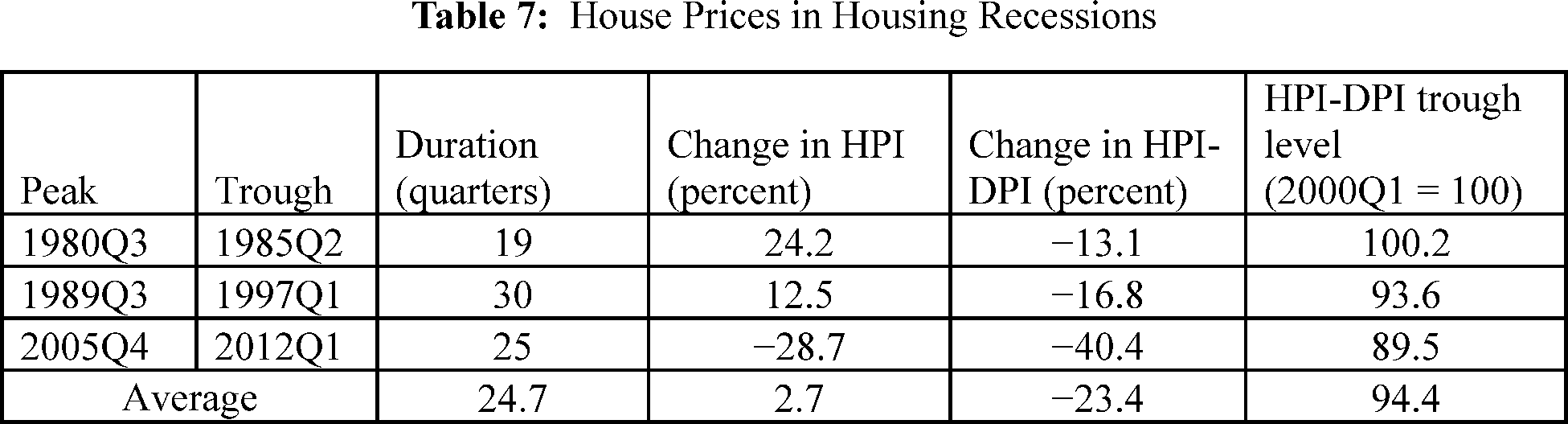
b. Additional Guide Parameters and Rationale

This subsection begins with a description of the construction of the house price series. This is followed by a description of the timing of the trough of HPI-DPI. The subsection concludes with information regarding the trajectory to trough.

Construction of House Prices From HPI-DPI

Unlike the guides for some other variables, such as unemployment and equity prices, this guide does not directly specify a path for house prices in the severely adverse scenario. Instead, this guide specifies a path for the HPI-DPI ratio. The scenario projection for house prices is then calculated from this ratio using paths for DPI and population, as calculated by the macroeconomic model for stress testing that the Board has developed specifically to aid in communicating the stress test scenario to the public specified on the Board's website. The scenario projection for population is the same as that contemplated in the Baseline Scenario Guide, as described in Section IX.C of this Supplementary Information and in section 4.1 of the Scenario Design Policy Statement. The scenario projection for house prices is then calculated as the HPI-DPI path, discussed in this guide, multiplied by nominal disposable income divided by population.

Trough Value Timing

In general, the entire 13-quarter trajectory of stress test variables is important as it ultimately affects implied firm losses. The Board expects that the trough of HPI-DPI typically should occur between quarter 8 and quarter 10 of the severely adverse scenario, as explained below.

To support this range for the timing of the trough in house prices, the Board applied the recession approach and used the timing of unemployment peaks to calibrate the timing of the trough of HPI-DPI. This benchmarking to the unemployment peak was necessary because house prices have more protracted cyclical dynamics than other scenario variables described in this framework. The three major house price retrenchments indicated in Table 7 featured peak-to-trough durations for HPI-DPI of between 19 and 30 quarters. The full implications of such a protracted decline cannot be adequately assessed by including only a portion of that decline within the nine-quarter horizon of the annual stress tests, because the resilience of firms would be impacted importantly by investors' perceptions of the expected future ( printed page 51891) losses.^[149] Moreover, the practical difficulties presented by the difference between the length of historical housing cycles and the length of the stress test scenario is an example of why the Board expects to maintain the flexibility to use scenarios that are not exactly like historical scenarios.^[150] Together, these two notions, one practical and the other principled, require the Board to consider a more careful approach to reading the historical record in its determination of the timing of the trough value for HPI-DPI.

Because the length of the severely adverse scenario cannot replicate the duration of historical housing recessions, the Board identified the subperiods within past housing recessions that featured the greatest declines in HPI-DPI to support its calibration of the trough within the scenario. This choice reflects the principle of severity. The Board considered three window lengths when calculating periods of maximum declines in HPI-DPI: 6, 9, and 13 quarters.^[151] The calculations in Table 7 include the trough-quarter of such windows, along with the percentage decline in HPI-DPI over each window.

Under the recession approach, the Board calibrates other variables to be consistent with the scenario path for unemployment. To compare the maximum decline in the HPI-DPI ratio with the peak in unemployment, the table also includes the timing of the peak quarter for unemployment along with the difference in timing between the peak unemployment rate and the end of the window. For example, when considering the period 2005Q4-2012Q1 (Column 3, Table 8), the 6-quarter window with the greatest change in HPI-DPI is 2007Q2-2008Q4 (Row 2, Column 3). This window featured a fall in the HPI-DPI ratio of 24.1 percent. The end of this window, 2008Q4 is 4 quarters before the unemployment rate peaked in 2009Q4.

On average, the quarter of the maximum decline in HPI-DPI over 6-quarter windows precedes the quarter of peak unemployment by 1.67 quarters. The unemployment guide features a range for the peak in unemployment with a midpoint in quarter 7. Therefore, to be consistent with some years' contemplated path for unemployment, a 6-quarter window for the decline in HPI-DPI would have to start with the scenario jump-off quarter rather than the first quarter of the scenario. Hence, the Board deemed a trough timing for HPI-DPI of 6 quarters as too short.

More promisingly, the relationship between the peak of unemployment and the trough of the HPI-DPI ratio flips at longer horizons. The unemployment peak quarter precedes the quarter of the maximum declines in HPI-DPI over 9 and 13 quarter windows by an average of 0.67 and 2.33, respectively. Therefore, trough timings of both 9 and 13 quarters would be broadly consistent with the length of the scenario and the timing of the unemployment peak within it. Of these two options, the Board deems that the trough timing of HPI-DPI should occur around quarter 9 for two auxiliary reasons: First, an interior trough time allows for some subsequent recovery, mirroring the movement of unemployment and other variables in this framework. Second, a shorter duration to trough, all else equal, will result in a more severe scenario, consistent with the principal of conservatism.

In addition, the maximum changes in HPI-DPI for the 6, 9, and 13 quarter subperiods associated with the 2007-2009 financial crisis are close to or larger than 25 percent. Hence, this subperiod analysis also further supports the calibration of the trough level in this guide.

Turning to a comparison with past scenarios, the selection of a range of quarter 8 to 10 for the trough of HPI-DPI in the severely adverse scenario is broadly consistent with the timing of past scenarios. In 2019 to 2022, the severely adverse scenario featured a trough in quarter 9. In 2023 to 2025, the severely adverse scenario featured a trough in quarter 7, as the Board assessed valuation pressures in residential real estate to be very elevated and wanted to ensure that the banking system remained resilient to a sudden correction in the housing market. Although that calibration of the guide would require the Board to explain its rationale for choosing an earlier trough going forward, the analysis presented above about the typical timing of house price troughs suggests that a trough between quarters 8 and 10 of the scenario usually would be sufficiently and credibly stressful. In choosing the timing of the trough, the Board expects to choose an earlier trough when the level of systemic risks is high or rising and a later trough when the level of systemic risks is low or declining. Housing market indicators such as recent trends in HPI-to-DPI ratios, house price growth, the growth rate of mortgage lending, or changes in mortgage lending standards are factors in that determination. Conversely, when vulnerabilities or risks related to residential real estate and related lending are low or decreasing, the Board could consider a later trough.

( printed page 51892)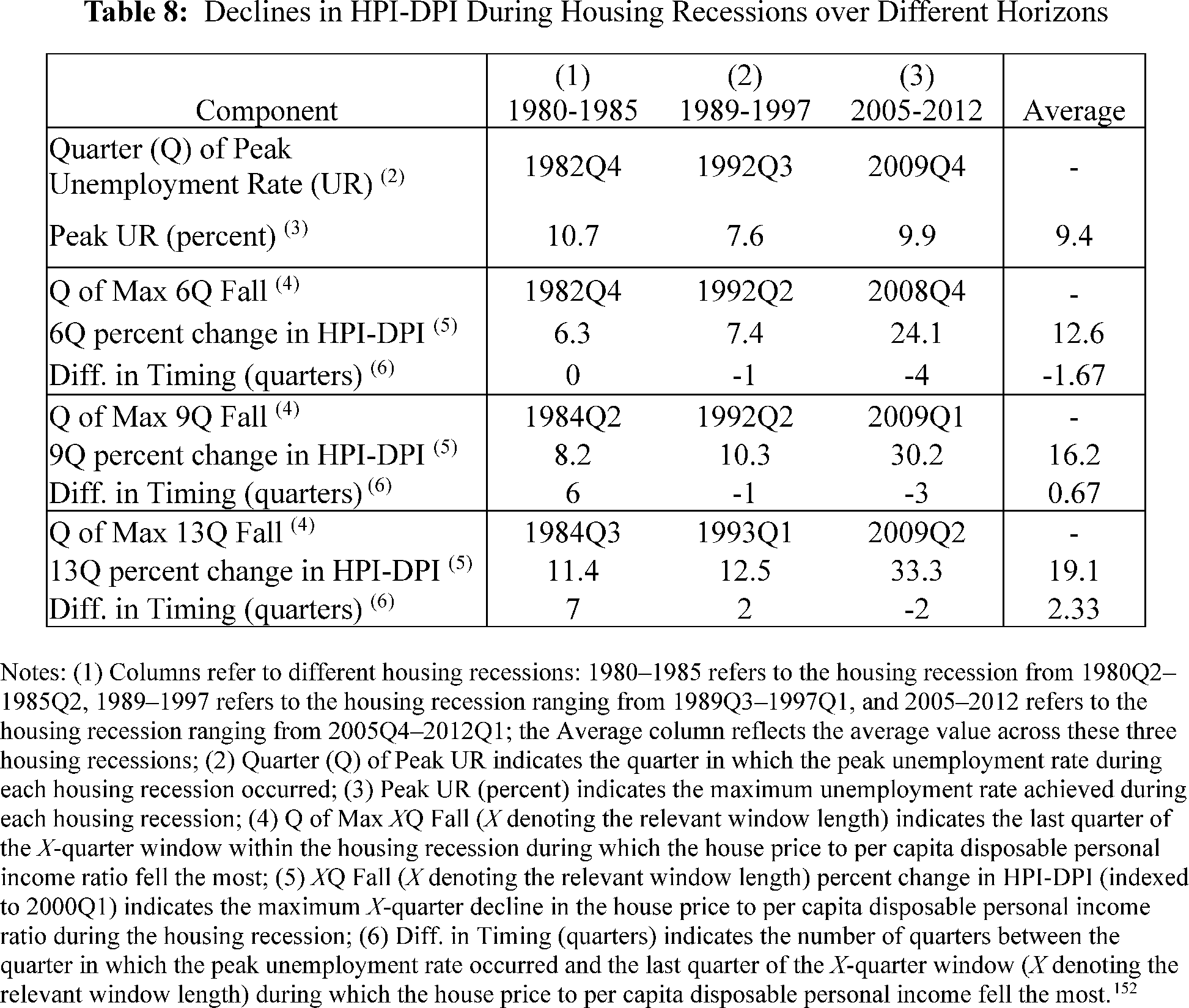

Trajectory to Trough

This guide specifies a trajectory to trough featuring 20 percent of the decline in the first quarter, 20 percent of the decline in the second quarter, and a linear trajectory to trough thereafter, subject to the rounding conventions mentioned in Section IX.F of this Supplementary Information. As shown in Table 8, housing recessions tend to be protracted. While the Board follows the recession approach, the other principles from the stress testing literature suggest that a careful reading of the data is warranted. To this end, when considering the windows with the most rapid declines in Table 8 above, further analysis shows that each housing recession featured quarters with declines near 20 percent. In an application of the principle of conservatism, the Board finds that two quarters of 20 percent declines broadly fits the scenario narrative of a rapid decline in economic conditions and sentiment, while meeting the other principles set out in this guide; frontloaded declines are relatively more severe, so are consistent with the principles of conservatism, severity, and the need to consider possibilities somewhat outside the historical evidence. The specification of linear declines thereafter was chosen in the interest of simplicity.

Moreover, a rapid decline in house prices is consistent with the recession approach, in which other variables in the scenario are guided by the scenario trajectory for the unemployment rate, which features rapid initial deterioration. In addition, rather than having HPI-DPI decline throughout the 13 quarter scenario as might be justified given the historical record, the Board expects that house prices in the severely adverse scenario will feature a moderate recovery after their trough—again, consistent with the recession approach where variables follow from the general movements of the unemployment rate, which itself recovers after its trough—a feature which moderates the severity of the initial decreases in house prices. Turning to past scenarios, a moderately frontloaded trajectory to trough strikes a balance between recent scenarios. Scenarios from 2023 to 2025 featured strongly frontloaded declines, with more than 40 percent of the drop happening in the first quarter, and increasingly smaller drops to the trough. Frontloading the decline in this manner is consistent with the principle of conservatism and the advice from stress testing literature to consider features that are outside of historical experience when vulnerabilities are elevated. The Board made a different decision with house price scenarios in 2021 and 2022, which featured a less stressful trajectory of initially small declines followed by a ( printed page 51893) period of larger declines while the economy was recovering from the COVID-19 recession. Hence, a moderately frontloaded trajectory falls between these earlier and later scenarios. The Board sees the reduction in flexibility in this component of the house price path as partially offset by the additional predictability and simplification that it provides.

The Board expects that a scenario consistent with the level, timing, and trajectory to the trough of house prices specified by this guide will be at least somewhat more severe than the average of past housing recessions and sufficiently close to the house price correction associated with the 2007-2009 financial crisis.

Commercial Real Estate Prices

The stress test scenarios set out trajectories for several variables, including commercial real estate prices as reported in the Board's Z.1 statistical release.^[153] The Commercial Real Estate Price Index aggregates price indices across office, retail, industrial and other types of properties.

In the supervisory stress test, commercial real estate prices capture a key part of the risks to firms from their commercial real estate exposures, which are reported by firms on FR Y-14Q, Schedule H.2. Most firms subject to the supervisory stress test have a substantial exposure to the commercial real estate market. Moreover, commercial real estate price build-ups often precede episodes of market stress. By incorporating commercial real estate prices into macroeconomic scenarios, supervisory stress tests help ensure that firms subject to the stress test are prepared for a range of market conditions, including periods of large decline in commercial real estate prices directly affecting the firms' balance sheets. This helps maintain the overall stability and resilience of the financial system.

In determining the appropriate level of scenario severity, the Board adheres to the scenario design principles discussed in the earlier Section IX.F of this Supplementary Information. While doing so, the Board also strives to avoid introducing additional sources of procyclicality into the financial system. In the context of commercial real estate prices, these principles are applied in calibrating three key aspects of the guide: the trough value, the timing of the trough value, and the trajectory to trough value. This approach ensures that the commercial real estate price guide aligns with the established stress testing literature while mitigating potential systemic risks for the financial system.

The rest of this section is organized as follows. First, Table 9 includes an overview of the Board's proposed guide for setting commercial real estate prices in the severely adverse scenario. The next subsection provides the data- and scenario-based rationale for the calibration of the trough component. Afterward follows a discussion of the alternative trough option, comparing the implementation and caveats to the proposed guide description. Finally, additional guide parameters for the trough timing and trajectory to trough value, and the rationale for their calibration are discussed.

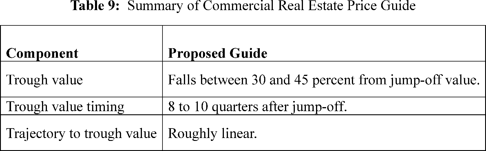
a. Trough Value Component of the Guide

The proposed guide stipulates that at the trough, commercial real estate prices will drop between 30 percent and 45 percent from the jump-off value. The choice of the specific magnitude of drop within this range will be determined based on the overall level of cyclical systemic risk and an assessment of relevant indicators in the market as reflected by a range of commercial real estate indicators such as the level and change over preceding years in commercial real estate prices, commercial real estate capitalization rate (cap rate), lending standards on commercial real estate loans, rents, and vacancy rates, among other indicators. The Board generally judges valuation pressures and the implied level of risk by looking at where recent observations of these relevant indicators are within their distributions.

Data- and Scenario-Based Rationale for the Trough Value

In line with the scenario design principles for setting the scenario severity, as discussed earlier in Section IX.F of this Supplementary Information, the proposed guide takes into account the dynamics of a variety of commercial real estate market indicators, including but not limited to the growth rates of commercial real estate prices, changes in bank lending standards in the commercial real estate segment, and the commercial real estate capitalization rate over the past several years. The consideration of several years of history for this variable is due to the slower-moving nature of commercial real estate markets, in contrast with market volatility (measured by the Chicago Board Options Exchange's CBOE Volatility Index (VIX)), stock market prices, and corporate bond spreads, as described in those guides below. The long-lived nature of these assets and substantial upfront financial investment involved can loosen the connections between their current observed valuations and financial conditions at firms and in broader financial markets. For instance, lending practices adopted in a period of declining prices, such as 2023 and 2024, can cloud immediate price signals. Additionally, the complexity of these connections and the ( printed page 51894) breadth of property types make it difficult to track developments in the commercial real estate sector with a single quantitative indicator or a very limited set of indicators that would constitute a basis for the commercial real estate guidance. Therefore, the proposed guide establishes a range of price decline values that determine the magnitude of the price decline to the trough, as well as its characteristics.

The proposed calibration of the range of decline (30 to 45 percent) to the trough for the commercial real estate price index is determined to account for commercial real estate price behavior in severe post-war U.S. recessions and to allow for increases in severity after economic expansions, in line with the principles outlined in the policy statement as well as those discussed earlier in this section. First, the range is centered around the value observed during the 2007-2009 financial crisis, when commercial real estate prices dropped about 39 percent from the peak in 2007Q3 to the trough in 2009Q4 (Table 10). Second, the extent of commercial real estate price upswings provides a guide for their subsequent unwinding and another target for the range. As mentioned in the Board's policy statement, cyclical vulnerabilities rise during more robust expansions. Looking back at the most recent commercial real estate cycle upswing in 2013-2024, the median four-year commercial real estate price growth rate in this period is about 30 percent, which the Board uses to calibrate the lower part of the range. Setting a floor for the decline in commercial real estate prices of 30 percent recognizes the fact that, not only do cyclical systemic risks build up at financial intermediaries during robust expansions, but also a minimum level of risk exists even in an already stressed environment. Separately, the Board opts for 45 percent as the higher end of the range, as a similar value (43 percent, as measured by the four-year growth rate of the commercial real estate price index between 2011Q3 to 2015Q3) was observed in the 2013-2024 commercial real estate cycle. The upper end of this range is also set to be larger than the 39 percent decrease experienced during the 2007-2009 financial crisis to allow for scenarios that feature commercial real estate price declines that are larger than what have been seen historically. Adequate severity requires a guide to be able to go somewhat beyond historical experiences when initial conditions warrant. Furthermore, certain sectors within the commercial real estate market have already experienced larger declines than 39 percent in the post-COVID-19 period, further justifying a range of potential declines that can address risks that are apparent in relevant indicators of economic and financial conditions as they arise.

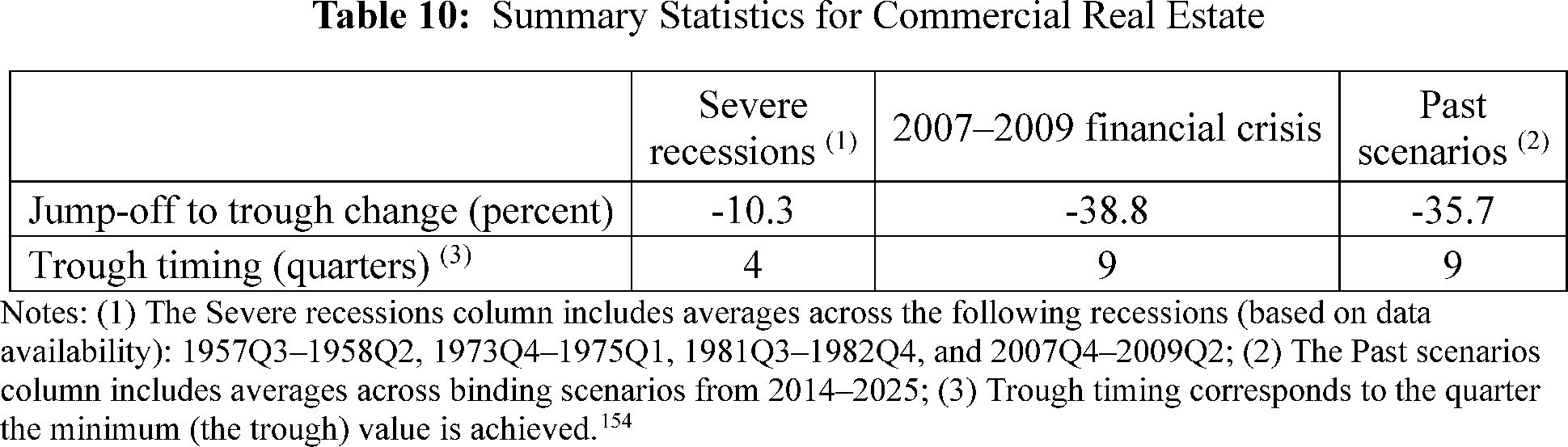
In its formulation of the annual scenarios, the Board could consider the overall level of cyclical systemic risk or various indicators related to commercial real estate markets to determine the appropriate decline in commercial real estate prices in the scenario. As discussed in Section IX.F of this Supplementary Information, the Board expects to calibrate the decline in commercial real estate prices based on its views of the status of cyclical systemic risk.

Specifically, the Board would be more likely to set the commercial real estate price trough value at the higher end of the range if the Board expects that cyclical systemic risks are high (as it would be after a sustained long expansion), and alternatively would be more likely to set the trough value to the lower end of the range if cyclical systemic risks are low (as it would be in the earlier stages of a recovery), provided doing so remained consistent with the goal of ensuring that firms were properly capitalized to withstand severe economic and financial conditions. This may result in a scenario that is more intense than normal if the Board expects that cyclical systemic risks were increasing in a period of sustained robust expansion.

Conversely, it would also allow the Board to specify a scenario that is less intense than normal in an environment where systemic risks appeared subdued, such as in the early stages of an expansion. This choice would consider that the scenario does not add unduly to remaining stress, thereby exacerbating the initial adverse shock, and it would be particularly appropriate if the Board judges that firms are already taking steps to reduce their risk—for instance, by potentially restricting lending to otherwise qualified borrowers. Factors such as whether underlying commercial real estate market conditions have started to normalize and higher-than-usual credit losses stemming from previous commercial real estate price declines were either already realized—or are in the process of being realized—and thus removed from firms' balance sheets would contribute to the assessment of cyclical systemic risks.^[155]

Figure 1 illustrates how the proposed guide (range between solid lines) performs compared to past scenarios (shown as dots). As seen in this figure, the proposed guide fully brackets the declines featured in previous scenarios. Thus, the proposed guide is likely to result in similar stress test severity as ( printed page 51895) before this revision to the policy statement.

Alternative Trough Guide Option

The Board considered an alternative trough option in which commercial real estate prices fall 35 percent from the jump-off value, or reversal of prior 4 years of price increases up to 45 percent, whichever results in a larger decline. The calibration of the alternative guide relies on the similar observations shown in Table 10 and used for the calibration of the proposed guide. Specifically, the alternative guide caps the decline in the commercial real estate prices to a range between 35 and 45 percent. However, to determine the specific decline in this range, in contrast to the proposed guide which considers a variety of commercial real estate-market indicators and allows for weighing them against each other, this alternative focuses on only one dimension of potential risks in the commercial real estate market—price pressures accumulated over the previous 4 years—and formalizes the decline to the trough based on this indicator.

The alternative guide stipulates that commercial real estate prices will decline to the trough from the jump-off value by 35 percent or by an amount needed to offset the four-year commercial real estate price growth preceding the jump-off quarter. Hence, the alternative minimum decline could be somewhat more severe compared to the proposed guide. That said, the decline is capped at 45 percent to constrain the trough calibration within historically plausible bounds. The choice of four years (rather than, for example, the one-year look back used in the equity price guide) to span the relevant accumulation period of price pressures for this guide stems from a slower-moving nature of the commercial real estate cycle, in contrast to faster moving variables (like VIX or stock prices). At the same time, choosing a longer look-back time period, such as five years, for example, would often produce commercial real estate growth rates above 45 percent, thus triggering the 45 percent maximum threshold of the guide too frequently and resulting in excessive scenario severity relative to historically observed events, particularly at the beginning of market corrections.^[157]

The commercial real estate price troughs set in past annual stress test scenarios and the prescription of the alternative guide could be noticeably different. In the data, previous commercial real estate price changes in annual stress test scenarios, the key factor in determining the prescription for the alternative guide, are not always highly correlated with other commercial real estate indicators that the Board would have used to gauge the extent of salient risks at the time.

For instance, from 2021-2023 (post-COVID-19 pandemic) the alternative guide would prescribe troughs at 35 percent below jump-off values, while the proposed guide would prescribe troughs similar to those of past scenarios, around 40 percent below jump-off. The alternative guide thus would not have accounted for the unusually small number of commercial real estate sales that occurred during that period and the upward biases in transaction-based commercial real estate ( printed page 51896) price indices created by the strategic behavior of owners, lenders, and buyers in those conditions.^[158] Once commercial real estate prices had declined considerably by 2024 and transaction volumes increased, the shallower trough calibration for this alternative guide aligns with the Board's choice for the severely adverse scenario.^[159] This example illustrates that focusing on only one quantitative indicator (four-year commercial real estate price growth) may be too narrow to determine an adequate severity for the magnitude of decline from the start of the stress test scenario to its trough ( i.e., start-to-trough decline) for this variable.

Therefore, a guide that weighs a broader range of indicators and how conditions differ by property type could provide a fuller, more adequate framework for the Board to choose an appropriate level of stress for commercial real estate exposures in future stress test scenarios. Consequently, the Board would consider the overall level of cyclical systemic risk, which is informed by a range of indicators related to commercial real estate markets, in its formulation of the annual scenarios as discussed in this section.

Although the proposed and the alternative guides are both discussed, and the Board views the alternative guide as reasonable, it may be insufficient to capture the complexity of the commercial real estate market relative to the proposed guide. In addition, the implementation of the alternative guide for commercial real estate would be complicated by the lack of a real-time commercial real estate price indicator. Typically, the data are available with a 4-month lag, which means that the final quarter or two of data required to compute the value of the guide would be based on a projection rather than reported data. The purpose of the alternative guide discussion is to invite comment on a reasonable alternative considered by the Board and to transparently lay out the Board's present arguments for choosing the proposed guide.

b. Additional Guide Parameters and Rationale Behind Them

Trough Timing

In general, the entire 13-quarter trajectory of stress test variables is important as it ultimately affects implied firm losses. The value of the trough and its timing signify the magnitude and timing of the most severe point in this trajectory. The Board considers the dynamics of commercial real estate prices using the official NBER recession dates augmented by one year prior to the beginning of the recession and one year after the end of the recession to compute summary statistics for validating the timing of the trough for commercial real estate prices in this guide. The Board considers such additional data points because of the slow-moving nature of the commercial real estate cycles, as referenced earlier in this section, in comparison with the fast-moving and forward-looking behavior of equity prices, corporate bond spreads, and VIX, for which the moves following the Lehman Brothers bankruptcy during the 2007-2009 financial crisis are most consistent with the scenario narrative adopted in this proposed policy statement.

The guide stipulates that the trough level in the scenario would be reached in quarters 8 to 10. This range is consistent with the slower-moving nature of commercial real estate price cycles, the practice in previous severely adverse scenarios, and the behavior in previous periods of financial stress or recession. In the stress episode surrounding the 2007-2009 financial crisis, the commercial real estate price trough was in quarter 9 (Table 10). The usual process of slow adjustment of commercial real estate prices and the ambiguity in the measurement of those prices described earlier in this section motivates the Board to reserve a range in which the adjustment occurs. Keeping the magnitude of the trough constant, a more delayed trough timing generally results in less severity of the overall path, as a less abrupt worsening in conditions and credit quality gives firms more time to adjust to the shock. Thus, a range in the timing (quarter 8 to 10) is an additional lever (together with the trough magnitude range) to avoiding the addition of sources of procyclicality in the stress test. The Board would likely consider a delayed timing of the trough when the cyclical vulnerabilities are lower, and an earlier trough timing when the Board deems it appropriate to increase scenario severity, as described in this section in relation to the choice of price decline.

Trajectory to Trough Value

To reach the trough value, the guide prescribes a smooth roughly-linear transition from the jump-off point to the trough. This prescription is consistent with the linear models often used in the statistical modeling of macroeconomic series.^[160] Commercial real estate prices are slower-moving, even in crisis times, so there is less evidence of the frontloading seen in faster-moving variables such as the VIX or BBB spreads. Moreover, the breadth of property types and lags in real-time data availability contribute to the difficulty of tracking the developments in this sector. As discussed above, transactions-based prices may have biases based on the strategic behavior of the parties involved. Given these circumstances, considering more complicated trajectories may inject unnecessary volatility into the exercise, counter to the principles laid out on effective stress testing in Quarles (2019).^[161]

The trajectories prescribed in previous scenarios are consistent with the proposed guidance that commercial real estate price declines are not frontloaded. The two exceptions are for the scenarios during 2017 and 2018, where the largest declines occur in the second quarter of the scenario. In these years' scenarios, to test the resilience of the banking system to strong economic conditions and commercial real estate price increases in prior years, the Board chose scenarios which called for deeper and earlier declines in commercial real estate prices than considered in prior years' stress test scenarios. Notwithstanding these exceptions, the smoother decline specified by the proposed guide is more in line with historical behavior of the series and has the benefit of reducing volatility.

Equity Prices

The stress test scenarios set out trajectories for several variables, including equity prices proxied by the U.S. Dow Jones Total Stock Market ( printed page 51897) Index (DWCF).¹⁶² This index includes about 3,700 stocks trading on U.S. exchanges that account for 95 percent of the total market capitalization.

Along with commercial real estate prices, housing prices, and the VIX, equity prices are an essential gauge for asset prices that affect the U.S. economy and the financial conditions of financial and nonfinancial firms. Equity prices are generally recognized as a leading indicator of future economic conditions broadly, including economic growth and inflation.¹⁶³ Therefore, testing the ability of a firm to withstand a steep decline in equity prices helps ensure that these firms are properly capitalized to withstand severe economic and financial conditions.

In the supervisory stress test scenarios, equity prices are converted to quarterly frequency using the quarter-end value. The Board's use of this aggregation method in the severely adverse scenario, rather than average or maximum value in the quarter used for other variables, is a deliberate choice that reflects how equity prices might impact the balance sheets of financial institutions. Quarter-end values provide a clear, specific point-in-time snapshot of market conditions, which is crucial for assessing firms' balance sheets and market risk exposures. For trading books and fair-value estimates for assets that firms hold, quarter-end prices provide the most up-to-date mark-to-market valuation, which is critical for stress testing. Equity markets are typically more liquid than debt markets or markets for real estate, which means the most recent prices are less likely to be affected by technical factors instead of economic fundamentals and expectations about future conditions than in bonds or property markets. Using quarter-end values also makes it easier to compare stress scenarios with historical data, which is often reported on a quarter-end basis. Finally, many equity options expire at the end of quarters, making quarter-end prices particularly relevant for assessing option-related risks.

In determining the appropriate level of scenario severity, the Board adheres to the scenario design principles discussed in the earlier Section IX.F of this Supplementary Information. While doing so, the Board also strives to avoid introducing additional sources of procyclicality into the financial system. In the context of equity prices, these principles are applied in calibrating three key aspects of the guide: the trough value, the timing of the trough value, and the trajectory to trough. This approach helps ensure that the equity price guide aligns with the established stress testing literature while mitigating potential systemic risks for the financial system.

The rest of this section is organized as follows. First, Table 11 summarizes all of the equity prices guide components. This is followed by a detailed description of the guide's trough component, including the data- and scenario-based rationale for the calibration of the trough component and a discussion of the alternative trough option. Finally, additional guide parameters and the rationale for their calibration are discussed.

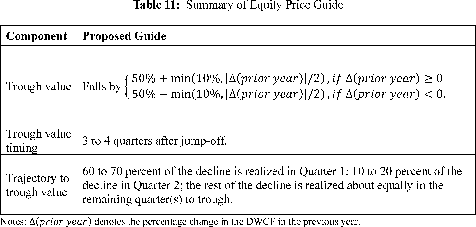
a. Trough Value Component of the Guide

The proposed guide stipulates that the decline in equity prices from the jump-off value ( i.e., the value of the equity price index at the end of the quarter immediately preceding the start of the scenario) will vary around 50 percent with an additional amount that offsets one half of the price growth over the prior year, up to 10 percent. These declines imply that equity prices would fall to a trough level that is between 40 and 60 percent below the jump-off value. More formally, this calibration implies that at the trough of the scenario path, equity prices fall by

( printed page 51898)

Data- and Scenario-Based Rationale for the Trough Value

In line with the scenario design principles for setting the scenario severity, discussed earlier in Section IX.F of this Supplementary Information, the rationale behind the choice of the neutral value of 50 percent comes from the data, as several recessions in the sample featured a decline of this magnitude. In particular, the equity price declines in the 1973 recession and the 2001 recession were 46 percent, whereas the decline in the 2007-2009 financial crisis measured 48 percent (Table 12). The equity price decline in the 2007-2009 financial crisis is most analogous to the scenario narrative, which starts with a substantial adverse shock to risk appetite and uncertainty and leads to a period of market disfunction followed by very high unemployment. Other financial stress episodes have seen maximum equity price declines of less than 50 percent, but in those instances the declines were not exacerbated by market dysfunction as considered in the scenario narrative.

The adjustment portion of this guide responds to the possibility that economic or financial conditions at the beginning of the annual stress test cycle might warrant a decline in equity prices that is smaller or larger than 50 percent. This flexibility reduces the likelihood that the calibration of the trough would unduly amplify rising or falling valuation pressures in equity prices over the past year. When the stock market does well (or poorly) in the prior year, the guide stipulates that equity prices fall by more (respectively, less), with the exact amount determined by one half of the prior year's price change. The use of half instead of, for example, full price change results in troughs that are less likely to be unduly severe. This calibration of the guide is based on historical equity market valuations. However, when recent price moves are not consistent with fundamentals or longer-term trends, the Board could deviate from the proposed guide and use price growth over a longer horizon.

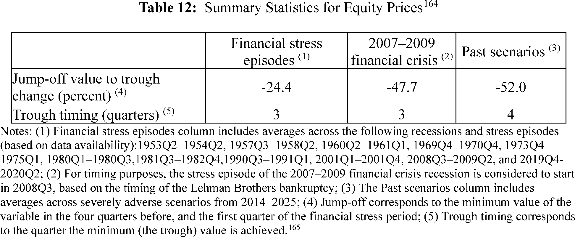
The choice of 10 percentage points as the upper bound for the absolute value of the year-to-year variation in this scenario variable, or equivalently the choice of effective bounds (between 40 and 60 percent) on the trough decline, is rooted in the data and is similar to changes that have been used in past severely adverse scenarios. The upper end of the range would allow the Board to meaningfully increase scenario severity when equity market valuations are likely to be high or rising (as they were during the dot-com era) to ensure that firms are resilient to outsized losses if valuations return to more normal levels. The lower end of the range would allow the Board to reduce scenario severity if equity valuation pressures recently declined, as might be the case following a stock market correction or early in an economic recovery.^[166] Setting a floor for the decline in equity prices of 40 percent recognizes the fact that, not only do cyclical systemic risks build up at financial intermediaries during robust expansions, but a minimum level of risk exists even in an already stressed environment.

Figure 2 illustrates how the proposed guide performs relative to the 2014-2025 stress test cycles, comparing the guide-implied decline with those of past stress test scenarios and realized changes in equity prices. Overall, the troughs implied by the proposed guide (solid line) are similar to past scenario ( printed page 51899) troughs. However, deviations between the proposed guide and past scenarios have been distributed across lower or higher severity, implying that the proposed guide and the previous more-judgmental process can provide similar average severity across multiple years of stress tests. Indeed, the decline in equity prices in past stress test scenarios during 2014-2025 averages 52 percent, whereas the proposed guide's prescription of the declines for the same period averages 55 percent. The slightly higher average decline is consistent with the principle of adequate severity discussed in Section IX.F of this Supplementary Information.

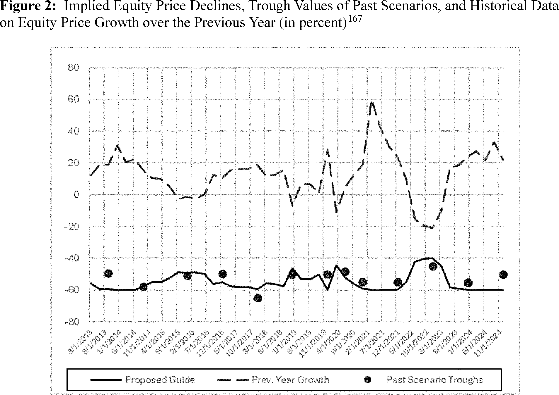
Alternative Trough Guide Option

The Board considered an alternative in which the trough would be a 50 percent decline from the jump-off value in equity prices unconditional on the previous year's price change and jump-off conditions. The 50 percent value is chosen based on the same reasons as the midpoint of the proposed guide. Although this alternative option is fully transparent and predictable, it has several weaknesses.

On average, the proposed guide would prescribe troughs that would have been somewhat lower than the alternative if it had been operational over the past 12 years: 55 percent for the proposed guide on average vs 50 percent for the alternative. However, although a 50 percent decline matches the judgmental average, it means that the test would be more severe each year than the decline observed during the 2007-2009 financial crisis.

Furthermore, as the alternative guide is not sensitive to the jump-off conditions, the resulting troughs could be either excessive or insufficient in severity, thus exacerbating procyclicality in ways the proposed guide does not. This weakness would be particularly detrimental to the credibility of the stress test during long bull markets (as the United States has experienced during the stress testing era) or periods of protracted decline in equity prices as the stress test would be serially under- or over-stating the likely risks.

The Board also considered a wider range in the proposed guide. An upper bound of 15 percentage points for the variable change relative to the midpoint of 50 percent would imply a much wider range of 35 to 65 percent declines at the trough. A 65 percent decline has not been observed in the post-war US data, whereas a 35 percent equity price decline could be insufficiently severe to maintain credibility of the test at times of heightened uncertainty. An upper bound of 5 percentage points for the variable change from the midpoint would cover the relevant historical benchmarks but would provide a narrow range: between 45 and 55 percent decline at the trough. This choice would substantially limit the Board's ability to match the severity of the equity price decline with the recent performance in equity markets so might inadvertently add to procyclical forces in financial markets. A choice of 10 percentage points as the upper bound on the change relative to the 50 percent midpoint strikes a balance between an overly narrow and an overly wide adjustment window.

Although the proposed and the alternative guides are both discussed, and the Board views the alternative guide as reasonable, the alternative guide's inability to respond to recent changes in equity valuations would be ( printed page 51900) a significant limitation compared with the proposed guide. The purpose of the alternative guide discussion is to invite comment on a reasonable alternative considered by the Board and to transparently lay out the Board's present arguments for choosing the proposed guide.

b. Additional Guide Parameters and Rationale Behind Them

Trough Timing

In general, the entire 13-quarter trajectory of stress test variables is important as it ultimately affects implied firm losses. The value of the trough and its timing signify the magnitude and timing of the most severe point in this trajectory. The guide stipulates that the trough level in the scenario would be reached in quarter 3 or quarter 4, which is consistent with historical observations (Table 12). For instance, in the stress episode surrounding the 2007-2009 financial crisis, the trough for equity markets occurred three quarters after the bankruptcy of Lehman Brothers in 2008Q3.^[168] That timing also accords with the scenario narrative, in which a sudden and significant increase in uncertainty and rapid deterioration in risk appetite leads to a spike in financial market volatility and a sharp decline in U.S. financial assets during the first quarter of the scenario.

Trajectory to Trough Value

To reach the trough value, the guide prescribes that between 60 and 70 percent of the decline occurs in the first quarter of the scenario, 10 to 20 percent of the decline occurs in the second quarter, with the remaining decline being realized about equally in the remaining quarter(s) to trough. This trajectory is consistent with the scenario narrative in which a severe recession is triggered by a large financial shock in the first quarter followed by a return to normal market functioning in subsequent quarters.

These expected trajectory benchmarks reduce the variation in trajectories relative to previous scenarios: across past severely adverse scenarios, the median first quarter decline in equity prices was 68.3 percent of the total decline, so a range between 60 and 70 percent is in line with the midpoint of past scenario choices. Also, across past severely adverse scenarios, the median second quarter decline in equity prices was 18.4 percent of the total decline, which is also within the range of 10 to 20 percent specified in this guide. Such a frontloaded decline is also consistent with the status of equity prices in the index of leading economic indicators and the empirical evidence from periods of equity market weakness.^[169] Across episodes of stock market distress, the average share of the decline realized in the two quarters preceding the trough amounts to 63 percent, with one episode measuring a much higher 88 percent in one quarter (in 1962) and most measuring 50 percent or more for these two quarters (for example, 52 percent in the 2007-2009 financial crisis).^[170]

In specifying a range for the timing of the trough and the proportion of declines in each quarter along the trajectory to the trough the Board maintains the option to create more or less severe scenarios if it wishes to avoid adding to existing procyclical factors or for another reason. An earlier trough with higher frontloading of the declines generally would be more severe. The Board could consider an earlier trough timing or higher frontloading when economic and financial market conditions are buoyant, such as when equity prices have increased by more than the maximum 10 percent adjustment to the trough level. A delayed trough timing and lower frontloading generally would decrease the scenario severity. The Board could consider delayed timing of the trough or smaller frontloading when equity prices at jump-off are depressed but have been increasing, or are projected to increase, and firms have de-risked and begun to recognize related losses.

VIX

The stress test scenarios set out trajectories for several variables, including the VIX, that is, the Chicago Board Options Exchange's CBOE Volatility Index. The VIX is an index measuring implied volatility based on a portfolio of options of the Standard and Poor's 500 (S&P 500).^[171] The VIX is calculated and distributed by the Chicago Board Options Exchange.^[172]

The VIX is often referred to as the “fear index” because it measures the market's expectation of future volatility. Furthermore, equity market volatility has been often used as an indicator of the price of risk, along with the spreads, which can depress economic activity when elevated.^[173]

In the supervisory stress test models that use the macroeconomic scenario, the VIX can act as an indicator of stress for a wide range of important assets and income streams even if those business lines are not specifically linked to the VIX index. By incorporating the VIX into scenarios, stress tests help ensure that firms are prepared for a wide range of market conditions, including periods of extreme volatility and uncertainty and any associated economic downturn.^[174] This helps maintain the overall stability and resilience of the financial system.

In the supervisory stress test scenarios, the VIX is converted to quarterly frequency using the maximum close-of-day value in any quarter and expressed in percent. The Board's use of this aggregation method in the scenarios, rather than average or quarter-end values as used for other variables, is a deliberate choice to have at least one scenario variable that reflects the unique nature of market volatility and its impact on financial institutions. This approach ensures firms are tested against the most extreme, potentially destabilizing market conditions, even if short-lived. Short-term and sharp increases in the VIX can reflect markets' initial response to changes in risk appetite or the economic outlook that then have longer-lasting adverse effects on the broader economy, such as reduced employment.^[175] Moreover, the use of the maximum close-of-day values captures the non-linear effects of volatility spikes on financial instruments, risk models, and liquidity, ( printed page 51901) while also testing firms' ability to handle rapid market movements, margin calls, and behavioral factors during peak stress.

In determining the appropriate level of scenario severity, the Board adheres to scenario design principles discussed in Section IX.F of this Supplementary Information. While doing so, the Board also strives to avoid introducing additional sources of procyclicality into the financial system. In the context of the VIX, these principles are applied in calibrating three key aspects of the guide: the peak value, the timing of the peak value, and the trajectory to peak. This approach ensures that the VIX guide aligns with the established stress testing literature while mitigating potential systemic risks for the financial system.

The rest of this section is organized as follows. First, Table 13 provides an overview of the VIX guide components, which is followed by the guide description of the peak component. A data- and scenario-based rationale for the calibration of the peak component follows in the next subsection. Next is a discussion of an alternative peak option, comparing the implementation and caveats to the proposed guide option. Finally, additional guide parameters and the rationale for their calibration are discussed.

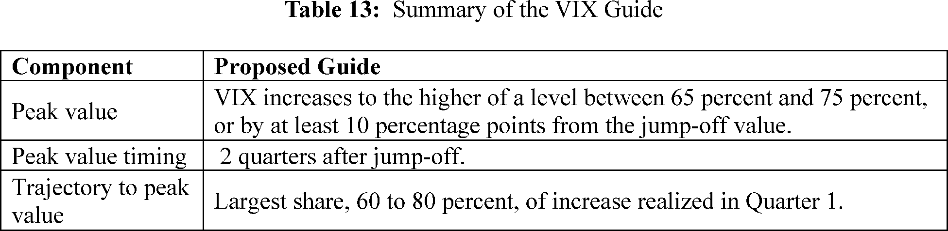
a. Peak Value Component of the Proposed Guide

The VIX will increase to a level between 65 percent and 75 percent or by at least 10 percentage points from the jump-off value, whichever results in a higher level.¹⁷⁶

Data- and Scenario-Based Rationale for the Peak Value

In line with the scenario design principles for setting the scenario severity, discussed in Section IX.F of this Supplementary Information, the VIX guide calibrates the minimum level to be between 65 percent and 75 percent. This choice is consistent with the historical observations during periods of stress (Table 14). In particular, the proposed range for the peak value of the guide is calibrated based mainly on the range of VIX realizations across four recent recessions or episodes of financial stress. The minimum value of 65 also reflects a judgment that the stress test always must be consistent with the goal of promoting financial stability, which means that markets and the public must continue to view the stress test as sufficiently severe to maintain confidence, especially during periods of high uncertainty and volatility.^[177] Thus, the lower end of the range for the guide is chosen to be modestly above the average VIX peak of 61 percent (first column). Moreover, setting a floor for the increase in the VIX of 65 percent recognizes the fact that, not only do cyclical systemic risks build up at financial intermediaries during robust expansions, but a minimum level of risk exists even in an already stressed environment. The higher end of the range is close to the maximum value across those periods, 83 percent, which was observed during the COVID-19 pandemic (third column).

( printed page 51902)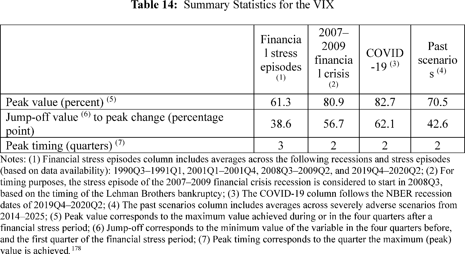

The minimum increment of 10 percentage points would only be relevant if the jump-off occurred during a period of already-high volatility (for example, in the 2007-2009 financial crisis, when the peak was 81 percent, or in the COVID-19 pandemic, when it was 83 percent). In such an instance, the guide allows for the possibility that conditions could worsen further, given the other aspects of the severely adverse scenario, such as the increase in unemployment and decline in house prices from the baseline. This assumption ensures that the VIX scenario peak is adequately severe. Limiting the increase to 10 percentage points ensures, however, that the peak does not deviate too far from historically observed levels and become unduly contractionary.

Figure 3 plots historical VIX data, past scenario peaks, and this guide (solid lines). On average across the past stress test scenarios (2014-2025), the VIX has been approximately 30 percent at the jump-off quarter, i.e., the data observation serving as a starting point for the scenario. The implied increase from the initial condition to the peak can be quite large—in such instances where the VIX is around 30 percent at the jump-off quarter, the increase to the peak value would be between 35-45 percentage points. Such rapid increases in the VIX are consistent with what occurred during the four stress episodes considered in this calibration. On average across those episodes, which start in 1990Q1 when data for the VIX became available, the VIX increases by approximately 39 percentage points from the onset of a stress event, which is one quarter before the start of the NBER recession date, to its peak, a value within the range implied by the guide (see Table 14, first column).

( printed page 51903)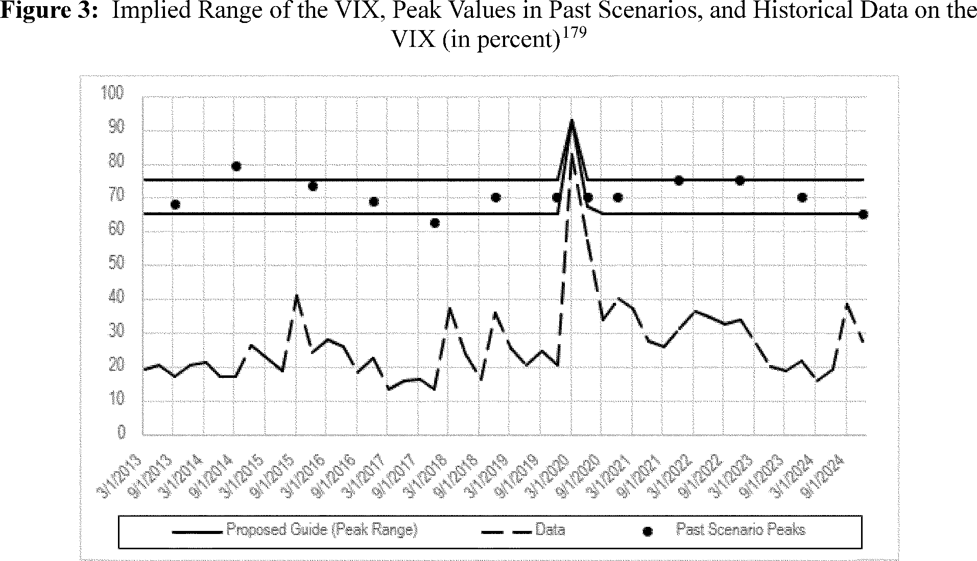

Figure 3 illustrates the comparison of the guide-implied peak range of the VIX (delineated by the solid lines) against the peaks in past stress test scenarios (shown as dots), accompanied by the respective jump-off points from the data (dashed line). Two key results emerge. First, past peaks chosen by the Board in previous severely adverse scenarios are mostly within the bounds that would have been stipulated by the VIX guide. In the two instances where the Board would have been more constrained, one episode was higher than the upper bound and the other lower than the lower bound. Thus, the guide is likely to result, on average, in similar stress test severity as before this revision to the policy statement while having the benefit of each individual year's scenario being more transparent and predictable. Second, the flexibility in the proposed guide to have a minimum increase of 10 percentage points provides adequate severity during stressful times, even beyond the upper end of the range for typical jump-off quarters. For instance, in 2020Q1, when the COVID-19 pandemic unfolded and the VIX jumped, reaching the historical maximum of the VIX, the prescribed peak would have been higher than 75 percent. Given the severity of the underlying conditions in 2020Q1, the peak would be determined by the jump-off point and the 10-percentage-point increment, resulting in a peak of 93 percent.

In its formulation of the annual scenarios, the Board's considerations would include the overall level of cyclical systemic risk, the current level of the VIX as a contemporaneous indicator of uncertainty and financial stress, and the performance of equity prices within the past 12 months as a forward-looking indicator of economic and financing conditions to determine the appropriate increase in the VIX in the scenario. As discussed in Section IX.F of this Supplementary Information, the Board expects to calibrate the increment in the VIX based on its views of the status of cyclical systemic risk. Specifically, the Board would be more likely to set the VIX peak value at the higher end of the range if the Board expects that cyclical systemic risks are high (as it would be after a sustained long expansion), and alternatively would be more likely to set the peak value to the lower end of the range if cyclical systemic risks are low (as it would be in the earlier stages of a recovery), provided doing so remained consistent with the goal of ensuring that firms were properly capitalized to withstand severe economic and financial conditions. This may result in a scenario that is more intense than normal if the Board expects that cyclical systemic risks were to be increasing in a period of sustained robust expansion. Conversely, it would also allow the Board to specify a scenario that is less intense than normal in an environment where systemic risks appeared subdued, such as in the early stages of a recovery. This choice would consider that the scenario does not add unduly to remaining stress, thereby exacerbating the initial adverse shock. The lower end of the increase range could also be appropriate when underlying market uncertainty and financial stress start to recede and higher-than-usual credit losses stemming from previously elevated vulnerabilities were either already realized—or are in the process of being realized—and thus removed from firms' balance sheets.^[180]

Alternative Peak Guide Option

The Board considered an alternative in which the VIX would increase to 75 percent or by at least 10 percentage points from the jump-off value, whichever results in a higher level. In this alternative peak option, the VIX would be set at a level of 75 percent in typical future scenarios. This prescriptive implementation would follow the principle of conservatism by always moving the VIX close to its historical maximum. It would also have the benefit of increasing the predictability of the guide. However, when the VIX at the jump-off value is elevated but has been declining or is ( printed page 51904) projected to decline and firm balance sheets are recovering, this alternative would remove the Board's discretion to choose a lower peak for the VIX. A lower but still constant value for the VIX guide in a typical scenario, for instance with a lower bound of 65 percent (corresponding to the average value across past scenarios) might not provide sufficient resilience in normal times, as the actual peaks of the VIX in the 2007-2009 financial crisis and during the COVID-19 pandemic exceeded 80 percent. Although a lower anchor could be coupled with a higher minimum increment value—for example, 20 percentage points—such a large increment in already stressful times removes the Board's discretion to choose a less severe VIX peak. Although the proposed and alternative guides are discussed, and the Board views a more restrictive alternative guide as potentially reasonable, the Board believes the alternative guide is inferior to the proposed guide, given the variation in peak levels of the VIX the Board has found appropriate in past stress test scenarios. Nonetheless, the purpose of the alternative guide discussion is to invite comment on a reasonable alternative considered by the Board and to transparently lay out the Board's present arguments for choosing the proposed guide.

b. Additional Guide Parameters and Rationale Behind Them

Peak Timing

In general, the entire 13-quarter trajectory of stress test variables is important as it ultimately affects implied firm losses. The value of the peak and its timing signify the magnitude and timing of the most severe point in this trajectory. The guide stipulates that the peak level in the scenario would be reached in quarter 2, which is consistent with past severely adverse scenarios and historical observations. The peak was reached in quarter 2 in both the 2007-2009 financial crisis and in the COVID-19 pandemic (see Table 14).^[181] Averaging across all four financial stress episodes used to calibrate the guide yields a peak in quarter 3. As historical maximum values of the VIX were reached in the 2007-2009 financial crisis and during the COVID-19 pandemic, and the scenario narrative specifies that the event is triggered by a financial crisis similar to events in the fall of 2008, the Board considers the peak timing in quarter 2 more appropriate for both the proposed and the alternative guide.

Trajectory to Peak Value

To reach the peak value, the guide prescribes that the highest share, 60 to 80 percent, of the VIX increase occurs in the first quarter of the scenario. Such frontloading of the increase is broadly consistent with empirical evidence and with the behavior of the other fast-moving variables (such as equity prices) in the scenario. Additionally, the academic literature considers the VIX (and other measures of uncertainty) a contemporaneous stress indicator that can respond to shocks on impact and stresses the importance of contemporaneous feedback between uncertainty and financial conditions.^[182] For instance, 100 percent of the increase in the VIX occurred in the first quarter of the 1990Q3-1991Q1 recession. During the 2007-2009 financial crisis, nearly 40 percent of the increase in the VIX occurred in the first quarter.^[183] In specifying a target for the proportion of increase to be realized in the first quarter, the Board would follow the same approach that it would use to assess appropriate severity for the peak value. In particular, during economic booms, the Board might formulate a scenario with greater frontloading of the VIX increases, as the scenarios with greater frontloading would contribute to higher severity. In the case of an economy that is characterized by moderate or slowing economic growth, the Board would likely stipulate the middle of the range of the VIX increases. Whereas in economic downturns or at the beginning of a recovery, the Board would expect to formulate a scenario with less frontloading of the VIX increases.

5-Year Treasury Yield

The stress test scenario sets out trajectories for several variables, including the 5-year Treasury yield, which is measured using the quarterly average of the yield on 5-year U.S. Treasury notes.^[184]

Because banks generally engage in maturity transformation by borrowing short-term ( i.e., deposits) to fund longer-term assets, fluctuations in interest rates can affect their financial health in various ways.^[185] The 5-year Treasury yield is an important benchmark rate for credit markets and is, thus, directly related to the profitability of banks' investments in loans and securities as well as their trading activities. For example, a decline in longer-term Treasury yields that exceeds the decline in short-term yields (known as a flattening of the yield curve) tends to compress firms' net interest margins and can therefore reduce their profitability. At the same time, the decline in such yields tends to increase the market value of firms' investments in long-term fixed-rate bonds, some which is reflected in various measures of capital at firms.^[186] Incorporating the 5-year Treasury yield into the supervisory stress test helps to ensure that firms are prepared for a wide range of market conditions, including periods with a sudden decline in a credit market benchmark rate. This helps maintain the overall stability and resilience of the financial system.

The Board uses a quarterly average of the 5-year Treasury yield in the stress test scenarios. Quarterly averages smooth out excessive (and potentially irrelevant) volatility that is present at daily or even monthly frequencies. Using quarterly averages strikes a balance between being sensitive enough to capture market trends and stable enough to avoid overreaction to market noise. Relatedly, the 5-year yield reflects long-term expectations of overall economic conditions. Therefore, removing short-term volatility from this measure via quarterly averaging is likely to, more-often-than-not, result in a ( printed page 51905) better representation of macroeconomic conditions.

In determining the appropriate level of scenario severity, the Board adheres to scenario design principles discussed in Section IX.F of this Supplementary Information. While doing so, the Board also strives to avoid introducing additional sources of procyclicality into the financial system. In the context of the 5-year yield, these principles are applied in calibrating three key aspects of the guide: the trough value, the timing of the trough value, and the trajectory to trough. This approach ensures that the 5-year yield guide aligns with the established stress testing literature while mitigating potential systemic risks for the financial system.

The rest of this section is organized as follows. First, Table 15 presents an overview of the 5-year Treasury yield guide components, followed by the guide description of the trough component. The next subsection provides the data- and scenario-based rationale for the calibration of the trough component. A discussion of an alternative trough option follows in the next subsection, comparing the implementation and caveats to the proposed guide option. Finally, additional guide parameters (trough value timing and trajectory to the trough) and the rationale for their calibration are discussed.

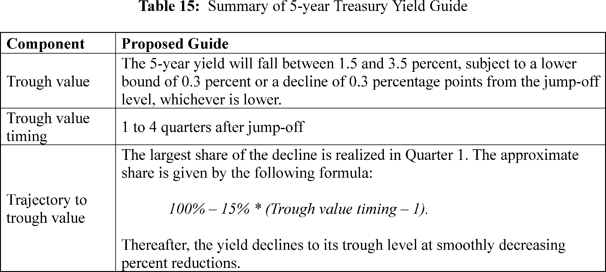
a. Trough Value Component of the Proposed Guide

Under the proposed guide, the 5-year Treasury yield decreases from its starting value by 1.5 to 3.5 percentage points. The Board expects to determine the size of the scenario's decline based on relevant banking, macroeconomic, or other conditions in the economy or financial markets.^[187] Additionally, the size of the decline will likely be informed by (a) the behavior of short-term interest rates in the macroeconomic model for stress testing that the Board has developed specifically to aid in communicating the stress test scenario to the public,^[188] (b) estimates of the likely term premiums in a period of economic weakness consistent with the scenario narrative, and (c) risks that are apparent in relevant indicators of economic and financial conditions.^[189] However, the guide restricts the 5-year Treasury yield from falling below a lower bound of 0.3 percent or a decline of 0.3 percentage points from the jump-off level, whichever is lower.

Data- and Scenario-Based Rationale for the Proposed Trough Value

In the recession approach chosen by the Board, risk-free long-term interest rates fall because reduced economic activity and inflation result in an easing of monetary policy. As noted above, declining interest rates can have both positive and negative implications for firms' capital levels, depending on the firm's business model and the specific composition of its assets and liabilities at the start of the stress test.

In line with these guiding principles as well as those emphasized by the stress testing literature discussed in Section IX.F of this Supplementary Information, the Board considers the behavior of the 5-year Treasury yield during four financial stress episodes since the mid-1980s, including the 2007-2009 financial crisis, to calibrate the guide (Table 16).^[190] The average decline in the 5-year Treasury yield ( printed page 51906) during those financial stress episodes has been around 2.7 percentage points, ranging from 2.1 to 3.5 percentage points.^[191] Notably, the percentage-point decline in the 5-year yield across these recessions is consistent even though the level of the yield at the start of the period has varied considerably.

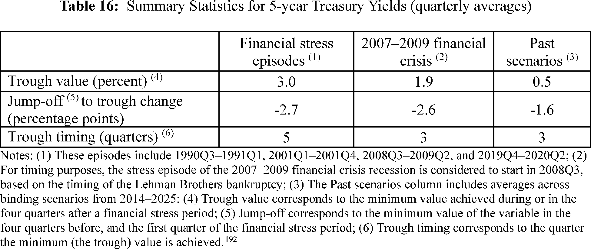
The evidence from the historical stress episodes along with the principle of conservatism and the goal of avoiding the addition of sources of procyclicality suggest that a decline of 1.5 to 3.5 percentage points in the 5-year Treasury yield would be reasonable. The lower end of the range ( i.e., 1.5 percentage points) is somewhat below the historical average decline in the yield during financial stress episodes and in previous severely adverse scenarios (Table 14), leaving room to adjust the decline—and thus severity of the scenario—relative to the historical average. The 5-year yield declined by 2.1 percentage points during the 1990Q3-1991Q1 recession.

The higher end of the range for the decline ( i.e., 3.5 percentage points) is driven by observations in the data as well as the guiding principles: first, the largest decline in the 5-year yield during NBER recessions since the mid-1980s has been 3.5 percentage points. This decline took place during the 2001Q1-2001Q4 recession. However, outside recessions, there are episodes displaying more sizable drops in the 5-year yield over the horizon of 13 quarters (matching the scenario horizon), the declines ranging from 2.6 to 6.1 percentage points. In particular, the episode spanning 1984Q2-1987Q2 had a drop of 6.1 percentage points, the episode spanning 1990Q3-1993Q3 had a drop of 3.5 percentage points, and the episode spanning 1999Q4-2002Q4 had a drop of 3.1 percentage points. These observations suggest that a decline of 3.5 percentage points in the 5-year yield is coherent with past experiences. Second, allowing the 5-year yield to potentially fall more than what has been observed, on average, during past recessions speaks to the guiding principle that adequate severity might sometimes require a scenario that is somewhat beyond typical historical experiences.

The guide also imposes a 0.3 percent lower bound for the value of the 5-year Treasury yield. The Board opted for this near zero, albeit positive, lower bound for a few reasons. First, the lower bound is intended to limit the extent that an annual scenario may unduly disincentivize bank lending when the economy is entering or recovering from a severe downturn. Second, this choice increases the predictability of the 5-year Treasury yield path in the scenario. Third, the lower bound is calibrated to be in line with the historical episodes. The 5-year Treasury yield declined to similar levels during the COVID-19 pandemic, reaching 0.3 percent in 2020Q3. Finally, the guide imposes a decline of 0.3 percentage points in the yield when the jump-off value of the 5-year yield is close to or below its historical minimums at the scenario jump-off. In particular, this element binds when the yield is below 0.6 percent at the jump-off. This element further increases transparency on the yield trough level in the scenarios in various potential interest rate environments outside historical experiences.

To illustrate how the trough levels of scenarios consistent with this guide would compare to the past stress test scenarios, consider the history of the 5-year yield and its scenario values at the trough over the period in which the Board has been conducting annual stress tests, from 2014 to 2025 (Figure 4). The past stress test scenario troughs are depicted as dots, whereas the range that is spanned by the proposed guide is indicated by the solid lines, incorporating the lower bound. The dashed line depicts the quarterly average of the 5-year Treasury yield observed in the data. This period contains both low- and high-interest rate environments: The quarterly average of the 5-year Treasury yield over that period was 2.1 percent, ranging between 0.3 and 4.5 percent at the jump-off quarter.

( printed page 51907)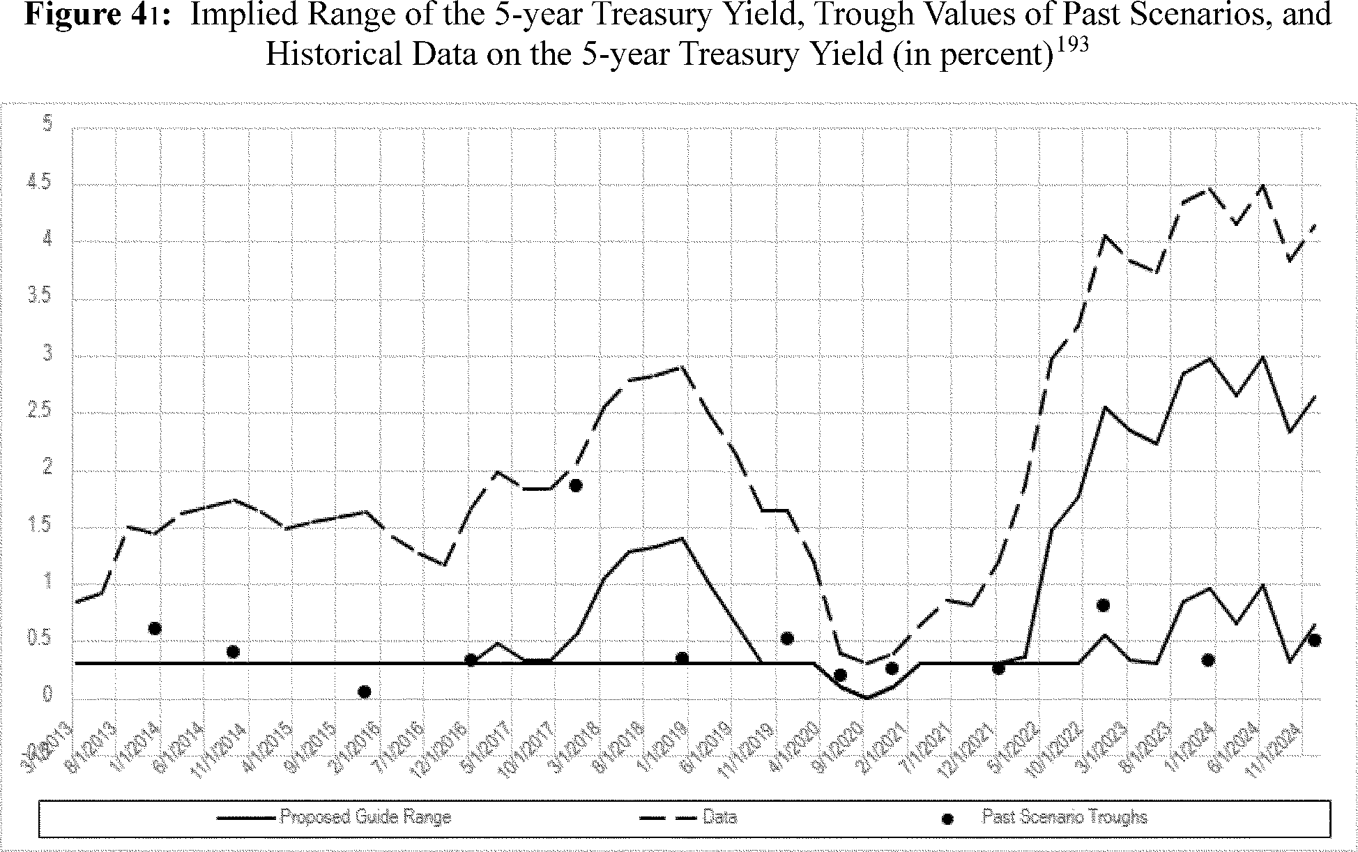

During the periods in which the 5-year yield was below 1.7 percent, such as most quarters between 2013 and 2016, and 2020 to 2021, the guide would prescribe the lower bound for the 5-year yield. In a higher-rate environment, however, a severe drop in the 5-year yield would not necessarily imply a yield close to zero, which the guide takes into an account. Between 2017Q1 and 2019Q2, the interest rate environment was such that the decline in the yield within the range of 1.5 to 3.5 percentage points would have provided the Board with the discretion to choose trough levels in the range of 0.3 and 1.4 percent. After 2022Q1, the proposed guide would have constrained the Board at times to a choice of yield levels significantly greater than the 0.3 percent lower bound.

Figure 4 also illustrates that the troughs implied by the proposed guide are quantitatively close to, but not the same as those featured in the past stress test scenarios during the low-interest-rate environment from 2013 to 2022 (the dots are located closer to the binding lower bound in most years). In several of those years, the Board chose a level for the trough that was modestly above the level that would have been prescribed by the guide and in one case the Board chose a level below the guide. However, with interest rates having risen to moderate levels between 2023 and 2025, the guide would have required the Board to choose a higher trough in 2024 and 2025 than it did.

The Board considers these deviations from past scenarios to be an acceptable consequence of adopting the guide, given its goal of increasing predictability and transparency in the stress test. On the one hand, a more flexible guide, which would encompass a higher share of the past scenario troughs both in the lower and higher interest rate environments, would call for a wider range in the variable component of the guide. While a wider range would increase scenario flexibility, it would come at the expense of predictability. The proposed range strikes a balance between providing an adequate amount of flexibility to allow for adjusting scenario severity based on economic and financial conditions and keeping scenarios predictable. On the other hand, keeping the range as is, one could also consider shifting the range up or down to better enclose the past scenario troughs. If the range was shifted down ( e.g., 1.0 to 3.0 percent), the guide would better encompass the past scenario troughs during the low-interest-rate periods, but the opposite would be true for the post-COVID-19 periods. If the range was shifted up ( e.g., 2.0 to 4.0 percent), the guide would better encompass the past scenario troughs between 2023 and 2025, but the lower bound would bind for a larger number of scenario troughs between 2013 and 2021. Thus, shifting the range would not meaningfully change how well the guide aligns with the past scenario troughs. Lastly, as the deviations from past scenarios would have been in both directions, the Board expects that the proposed guide will be broadly consistent with maintaining an average level of severity of stress tests going forward that is similar to what it has been under the Scenario Design Policy Statement.

In setting the 5-year Treasury yield trough value, the Board could consider the overall level of cyclical systemic risk, and the current level of the 5-year Treasury yield as a benchmark measure of overall economic and financing conditions. As discussed earlier in Section IX.F of this Supplementary Information, the Board expects to calibrate the increment in the 5-year yield in consideration of observable cyclical systemic risk. The Board would also consider how declines in Treasury yields, which decrease net income but increase the market value of firms' long-term securities holdings, interact with the current vulnerabilities in the banking sector. In general, a decline in long-term interest rates may have a positive or negative effect on the severity of the scenario for a given firm ( printed page 51908) depending on the firm's exposure to interest rate risk, which may vary from year to year depending on the firm's portfolio. In reaching its determination to set this guide in an annual scenario, the Board will consider how the choice would promote stress test credibility and the resilience of the financial system to even worse outcomes. If the Board observes that cyclical systemic risks were increasing in a period of sustained robust expansion, the Board might choose a scenario that is more severe than normal. The choice would also depend on firms' exposure to interest rate risk. Conversely, the Board could specify a scenario that is less intense than normal in an environment where systemic risks appeared subdued, such as in the early stages of a recovery, provided that doing so remained consistent with the goal of ensuring that firms were properly capitalized to withstand severe economic and financial conditions. A less severe scenario could also be appropriate when underlying market uncertainty and financial stress start to recede and higher-than-usual credit losses were either already realized—or are in the process of being realized—and thus removed from firms' balance sheets. The choice would consider that the scenario does not add unduly to remaining stress, thereby exacerbating the initial adverse shock, and it would be particularly appropriate if the Board judges that firms are already taking steps to reduce their risk.^[194]

Alternative Trough Guide Option

As an alternative, the Board also considered a guide in which the 5-year Treasury yield would decline by 2.5 percentage points regardless of the jump-off conditions, with the lower bound still applying. Under this alternative, the decline of 2.5 percentage points is chosen based on the same observations shown in Table 16. In particular, 2.5 percentage points is close to the average decline in the 5-year Treasury yield observed during the financial stress episodes (2.7 percentage points). The choice of a single value in the middle of the range proposed in the proposed version of this guide reflects the offsetting effects of interest rates on net interest margin and fair value of securities.

The Board considered this alternative because of its goal of increasing transparency and predictability of the stress test, while maintaining sufficient severity. However, the Board recognizes that this alternative guide would not avoid adding sources of procyclicality as effectively as the proposed guide. In particular, it would reduce the Board's flexibility during periods of moderate or high interest rates to test the resilience of firms' net income to a sharper decline in interest rates. However, as noted above, declines in yields have offsetting effects on firms' regulatory capital in the stress test because they decrease net income but increase the market value of their long-term securities holdings. Thus, a more flexible guide could have more-balanced effects on the stress capital buffer calculated from the stress test results.

While the alternative troughs fall within the range determined by the proposed guide, these trough levels can be significantly higher or lower than the values chosen by the Board in prior severely adverse scenarios. These deviations could impair the Board's ability to ensure that the stress test severity fully considers the risks that are apparent in relevant indicators of economic and financial conditions, particularly those related to the Treasury term premium, when determining the trough value. The Board views the alternative guide as reasonable. As compared to the proposed guide, the alternative guide would provide firms and the public with increased predictability regarding the trough value to be set for 5-year Treasury yields. However, this increased predictability under the alternative guide comes at the expense of the added flexibility inherent in the proposed guide to set the trough based on risks that are apparent in relevant indicators of economic and financial conditions and to avoid adding sources of procyclicality in the proposed guide. The purpose of the alternative guide discussion is to invite comment on a reasonable alternative considered by the Board and to transparently lay out the Board's present arguments for choosing the proposed guide.

b. Additional Guide Parameters and Rationale Behind Them

Trough Value Timing

In general, the entire 13-quarter trajectory of stress test variables is important as it ultimately affects implied firm losses. The value of the trough and its timing signify the magnitude and timing of the most severe point in this trajectory. The proposed guide suggests that the 5-year Treasury yield would reach the trough between quarters 1 and 4 of the scenario. This timing is chosen such that the trough is consistent with the scenario narrative: the severely adverse scenario is triggered by a sizeable financial shock combined with a pronounced increase in unemployment and decrease in inflation. In response to these developments, both short- and long-term interest rates typically would fall sharply. The timing of the trough is also broadly consistent with the historical data (Table 16). Averaging across the four financial stress episodes, the trough is placed in the fifth quarter, but the trough occurred earlier during the two most recent recessions.^[195] The 5-year yield reached its trough in quarter 3 during the 2007-2009 financial crisis and in quarter 4 during the COVID-19 pandemic. In the past stress test scenarios, the trough was also reached in quarter 3, on average. In setting this part of the guide in an annual scenario, the Board expects to consider the same indicators and other factors described above for the choice of the trough in the 5-year rate, so as best to promote stress test credibility and the resilience of the financial system to even worse outcomes.

Trajectory to Trough Value

The proposed guide stipulates that the largest share of the decline in the 5-year Treasury yield would be realized in quarter 1. A rapid, frontloaded decline of the 5-year yield to its trough would be consistent with the scenario narrative and the implied dynamics of the other variables, mainly the large increase in unemployment and resulting declines in inflation and output. In response to these developments, both short- and long-term interest rates would fall sharply, consistent with the Board's macroeconomic model for stress testing, and specifically the expectational component of the 5-year Treasury yield, which accounts for the future expected realizations of the macro variables that determine the policy rate rule.^[196]

To determine the specific path of the 5-year Treasury yield for a given trough timing, the Board considered a simple formula that can map the trough value timing to a share of decline in quarter ( printed page 51909) 1. To do so, the Board considered lower and upper bound of trough timing described in the previous section. If the trough timing is quarter 1 ( e.g., lower bound of the range), then the formula should yield 100 percent of the decline occurring in the first quarter. For trough timing of quarter 4, the Board took example of COVID-19 pandemic. During the COVID-19 pandemic, the 5-year yield reached its trough in quarter 4, and nearly 50 percent of the decline in the 5-year yield was realized during the first quarter. Using these reference points, the Board concluded that the following simple formula could determine the approximate share of the decline realized in quarter 1 as:

100% − 15% * (Trough value timing − 1).

This simple formula stipulates that when the scenario trough is realized in quarter 4, about 55 percent of the decline would be realized in quarter 1:

100% − 15% * (4 − 1) = 55%

This result is broadly in line—if not exactly in line—with the data from the COVID-19 pandemic. The guide also stipulates that, after the initial decline realized in quarter 1, the yield declines to its trough at smoothly decreasing percent reductions.

10-Year Treasury Yield

The stress test scenarios set out trajectories for several variables, including the 10-year Treasury yield, which is measured using the quarterly average of the yield on 10-year U.S. Treasury notes.^[197] Because banks generally engage in maturity transformation by borrowing short-term ( i.e., deposits) to fund longer-term assets, fluctuations in interest rates can affect their financial health in various ways. The 10-year Treasury yield is an important benchmark rate for credit markets and is, thus, directly related to the profitability of firms' investments in loans and securities as well as their trading activities. For example, a decline in longer-term Treasury yields that exceeds the decline in short-term yields (known as a flattening of the yield curve) tends to compress firms' net interest margins and can therefore reduce their profitability. At the same time, the decline in such yields tends to increase the value of firms' investments in long-term fixed-rate bonds, some of which is reflected in various measures of capital at firms.^[198] Incorporating the 10-year Treasury yield into the supervisory stress test helps to ensure that firms are prepared for a wide range of market conditions, including periods with a sudden decline in a credit market benchmark rate. This helps maintain the overall stability and resilience of the financial system.

The Board uses a quarterly average of the 10-year Treasury yield in the stress test scenarios. Quarterly averages smooth out excessive (and potentially irrelevant) volatility that is present at daily or even monthly frequencies. Using quarterly averages strikes a balance between being sensitive enough to capture market trends and stable enough to avoid overreaction to market noise. Relatedly, the 10-year yield reflects long-term expectations of overall economic conditions. Therefore, removing short-term volatility from this measure via quarterly averaging is likely to, more-often-than-not, result in a better representation of current macroeconomic conditions.

In determining the appropriate level of scenario severity, the Board adheres to scenario design principles discussed in the earlier Section IX.F of this Supplementary Information. While doing so, the Board also strives to avoid introducing additional sources of procyclicality into the financial system. In the context of the 10-year yield, these principles are applied in calibrating three key aspects of the guide: the trough value, the timing of the trough value, and the trajectory to trough. This approach helps ensure that the 10-year yield guide aligns with the established stress testing literature while mitigating potential systemic risks for the financial system.

The rest of this section is organized as follows. First, Table 17 presents an overview of the 10-year Treasury yield guide components, followed by the guide description of the trough component. The next subsection provides the data- and scenario-based rationale for the calibration of the trough component. A discussion of an alternative trough option follows in the next subsection, comparing the implementation and caveats to the proposed guide option. Finally, additional guide parameters (trough value timing and trajectory to the peak) and the rationale for their calibration are discussed.

( printed page 51910)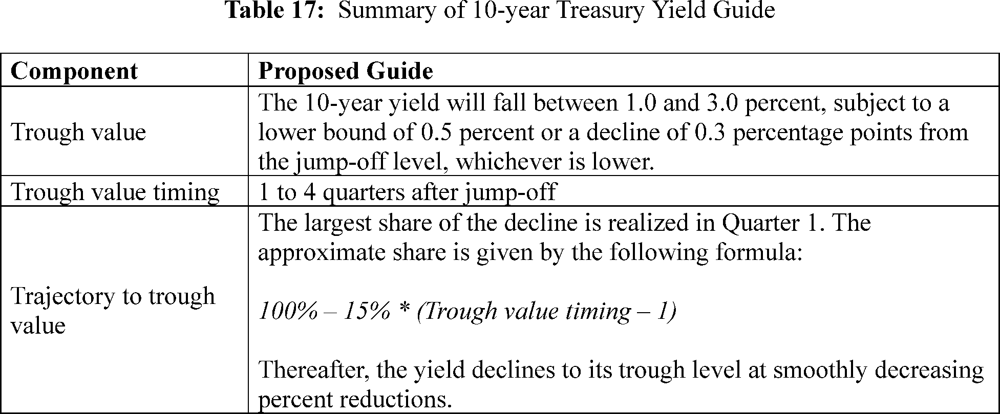

a. Trough Value Component of the Proposed Guide

The 10-year Treasury yield decreases from its starting value by between 1.0 to 3.0 percentage points. The Board will determine the size of an annual scenario's decline based on a number of factors, including relevant banking, macroeconomic, or other conditions in the economy or financial markets.^[199] Additionally, the size of the decline will be informed by (a) the behavior of short-term interest rates in the macroeconomic model for stress testing that the Board has developed specifically to aid in communicating the stress test scenario to the public,^[200] (b) estimates of the likely term premiums in period of economic weakness consistent with the scenario narrative, and (c) risks that are apparent in relevant indicators of economic and financial conditions.^[201] However, the guide restricts the 10-year Treasury yield from falling below a lower bound of 0.5 percent or a decline of 0.3 percentage points from the jump-off level, whichever is lower.

Data- and Scenario-Based Rationale for the Proposed Trough Value

In the recession approach chosen by the Board, risk-free long-term interest rates fall because reduced economic activity and inflation result in an easing of monetary policy. As noted above, declining interest rates can have both positive and negative implications for firms' capital levels, depending on the firm's business model and the specific composition of its assets and liabilities at the start of the stress test.

In line with these guiding principles as well as those emphasized by the stress testing literature discussed in Section IX.F of this Supplementary Information, the Board considers the behavior of the 10-year Treasury yield during four financial stress episodes since the mid-1980s, including the 2007-2009 financial crisis, to calibrate the guide (Table 18).^[202] The average decline in the 10-year Treasury yield during those financial stress episodes has been around 1.9 percentage points, ranging from 1.3 to 2.4 percentage points.^[203] Notably, the percentage-point decline in the 10-year yield across these recessions is similar even though the level of the yield at the start of the period has varied considerably.

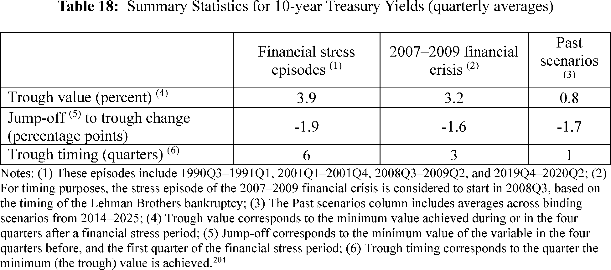
The evidence from the historical stress episodes along with the principle of conservatism and the goal of avoiding the addition of sources of procyclicality suggest that a decline of 1.0 to 3.0 percentage points in the 10-year Treasury yield would be reasonable. The lower end of the range ( i.e., 1.0 percentage points) is somewhat below the historical average decline in the yield during financial stress episodes and in previous severely adverse scenarios (Table 18), leaving room to adjust the decline—and thus severity of the scenario—relative to the historical average. The 10-year yield declined by 1.3 percentage points during the 1990Q3-1991Q1 recession.

The higher end of the range for the decline ( i.e., 3.0 percentage points) is driven by observations in the data as well as the guiding principles: first, the largest decline in the 10-year yield during NBER recessions since the mid- ( printed page 51911) 1980s has been 2.4 percentage points. This decline took place during both the 2001Q1-2001Q4 recession and the COVID-19 pandemic. However, outside recessions, there are episodes displaying more sizeable drops in the 10-year yield over the horizon of 13 quarters (matching the scenario horizon), the declines ranging from 2.2 to 5.8 percentage points. In particular, the episode spanning 1984Q2-1987Q2 had a drop of 5.8 percentage points, the episode spanning 1990Q3-1993Q3 had a drop of 3.0 percentage points, the episode spanning 1999Q4-2002Q4 had a drop of 2.2 percentage points, and the episode spanning 2018Q4-2021Q4 had a drop of 2.4 percentage points. These observations suggest that a decline of 3.0 percentage points in the 10-year yield is coherent with past experiences. Second, allowing the 10-year yield to potentially fall more than what has been observed during past recessions, on average, speaks to the guiding principle that adequate severity should be somewhat beyond historical experiences.

The guide also imposes a 0.5 percent lower bound for the value of the 10-year Treasury yield. The Board opted for this near zero, albeit positive, lower bound for a few reasons. First, the lower bound is intended to limit the extent that an annual scenario may unduly disincentivize bank lending when the economy is entering or recovering from a severe downturn. Second, this choice increases the predictability of the 10-year Treasury yield path in the scenario. Third, the lower bound is in line with the historical episodes. The 10-year Treasury yield declined to similar levels during the COVID-19 pandemic, reaching 0.6 percent in 2020Q3, but it has never fallen below that level. Finally, the guide imposes a decline of 0.3 percentage points in the yield when the jump-off value of the 10-year yield is close to or below its historical minimums at the scenario jump-off. In particular, this element binds when the yield is below 0.8 percent at the jump-off. This element further increases transparency on the yield trough level in the scenarios in various potential interest rate environments outside historical experiences.

To illustrate how the trough levels of scenarios consistent with this guide would compare to the past stress test scenarios, consider the history of the 10-year yield and its scenario values at the trough over the period in which the Board has been conducting annual stress tests, from 2014 to 2025 (Figure 5). The past stress test scenario troughs are depicted as dots, whereas the range that is spanned by the proposed guide is indicated by the solid lines, which incorporate the lower bound. The dashed line depicts the quarterly average of the 10-year Treasury yield observed in the data. This period contains both low- and high-interest rate environments, and the quarterly average of the 10-year Treasury yield (depicted as a dashed line) has been 2.5 percent, with a range between 0.6 and 4.5 percent at the jump-off quarter.

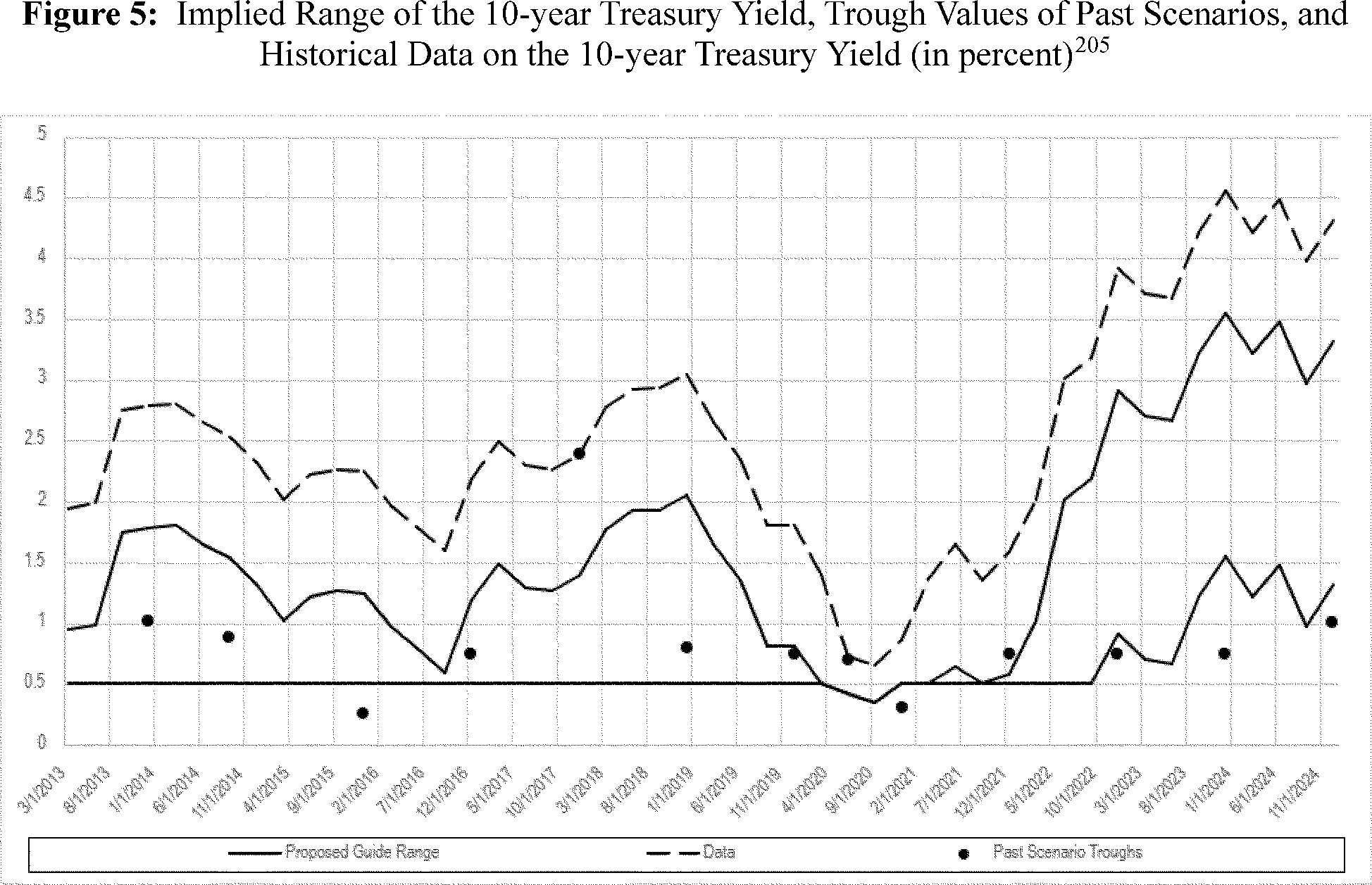
For periods when the 10-year yield is below 1.5 percent, such as the period surrounding the COVID-19 pandemic, the guide would prescribe the lower bound for the 10-year yield. In other periods between 2013-2025, the 10-year yield has been high enough such that the lower bound of the guide is not strictly binding after applying the minimum amount of decline in the guide. In a higher-rate environment, a severe drop in the 10-year yield would not necessarily imply a yield close to zero. Figure 5 illustrates that the range of troughs consistent with the proposed guide usually includes the values ( printed page 51912) featured in the past stress test scenarios during the low-interest-rate environment from 2013 to 2022 (the dots are located within the guide-prescribed range, or close to the binding lower bound in most years). In three of those years, the Board chose a level for the trough that was above the maximum level that would have been allowed by the guide and in two cases the Board chose a level modestly below the minimum level consistent with guide. With interest rates having risen to moderate levels between 2023 and 2025, the guide would have required the Board to choose a slightly higher trough in 2023 and 2025 and a notably higher trough in 2024 than the Board chose in those scenarios.

The Board considers these deviations from past scenarios to be an acceptable consequence of adopting the guide, given its goal of increasing predictability and transparency in the stress test. As the deviations from past scenarios would have been in both directions, the Board expects that the proposed guide will be broadly consistent with maintaining an average level of severity of stress tests going forward that is similar to what it has been under the previous scenario design framework.

In setting the 10-year Treasury yield trough value, the Board could consider the overall level of cyclical systemic risk, and the current level of the 10-year Treasury yield as a benchmark measure of overall economic and financing conditions. As discussed in earlier Section IX.F of this Supplementary Information, the Board expects to calibrate the increment in the 10-year yield in consideration of observable cyclical systemic risk. The Board would also consider how declines in Treasury yields, which decrease net income but increase the market value of firms' long-term securities holdings, interact with the current vulnerabilities in the banking sector. In general, a decline in long-term interest rates may have a positive or negative effect on the severity of the scenario for a given firm depending on the firm's exposure to interest rate risk, which may vary from year to year depending on the firm's portfolio. In reaching its determination to set this guide in an annual scenario, the Board will consider how the choice would promote stress test credibility and the resilience of the financial system to even worse outcomes.

If the Board observes that cyclical systemic risks were increasing in a period of sustained robust expansion, the Board might choose a scenario that is more intense than normal. The choice would also depend on firms' exposure to interest rate risk. Conversely, the Board could specify a scenario that is less intense than normal in an environment where systemic risks appeared subdued, such as in the early stages of a recovery, provided that doing so remained consistent with the goal of ensuring that firms were properly capitalized to withstand severe economic and financial conditions. A less severe scenario could also be appropriate when underlying market uncertainty and financial stress start to recede and higher-than-usual credit losses were either already realized—or are in the process of being realized—and thus removed from firms' balance sheets. The choice would consider that the scenario does not add unduly to remaining stress, thereby exacerbating the initial adverse shock, and it would be particularly appropriate if the Board judges that firms are already taking steps to reduce their risk—for instance, by potentially restricting lending to otherwise qualified borrowers.^[206]

Alternative Trough Guide Option

As an alternative, the Board considered a guide in which the 10-year Treasury yield would decline by 2.0 percentage points regardless of the jump-off conditions. The lower bound would still bind. The decline of 2.0 percentage points is chosen based on the same observations shown in Table 18. In particular, 2.0 percentage points is close to the average decline in the 10-year Treasury yield observed during the financial stress episodes (1.9 percentage points) and the average decline in previous severely adverse scenarios (1.7 percentage points). The choice of a single value in the middle of the range proposed in the more flexible version of this guide balances the offsetting effects of interest rates on net interest margin and fair value of securities.

The Board considered this alternative because of its goal of increasing transparency and predictability of the stress test, while maintaining sufficient severity. The Board recognizes that this alternative guide would not avoid adding sources of procyclicality as effectively as the proposed guide. In particular, it would reduce the Board's flexibility during periods of moderate or high interest rates to test the resilience of firms' net income to a sharper decline in interest rates. However, as noted above, declines in yields have offsetting effects on firms' regulatory capital in the stress test because they decrease net income but increase the market value of their long-term securities holdings. Thus, a more flexible guide would allow the Board to balance its assessment of these two vulnerabilities in the stress test scenario.

While the alternative troughs fall within the range determined by the proposed guide, these trough levels can be significantly higher or lower than the values chosen by the Board in prior severely adverse scenarios. These deviations could impair the ability of the Board to ensure the stress test severity that fully considers the risks that are apparent in relevant indicators of economic and financial conditions, particularly those related to inflation and inflation expectations, when determining the trough value. The Board views the alternative guide as reasonable. Compared to the proposed guide, the alternative guide would provide firms and the public with increased predictability regarding the trough value to be set for 10-year Treasury yields. However, this increased predictability under the alternative guide comes at the expense of the added flexibility inherent in the proposed guide to set the trough based on risks that are apparent in relevant indicators of economic and financial conditions and to avoid adding sources of procyclicality in the proposed guide. The purpose of the alternative guide discussion is to invite comment on a reasonable alternative considered by the Board and to transparently lay out the Board's present arguments for choosing the proposed guide.

b. Additional Guide Parameters and Rationale Behind Them

Trough Value Timing

In general, the entire 13-quarter trajectory of stress test variables is important as it ultimately affects implied firm losses. The value of the trough and its timing signify the magnitude and timing of the most severe point in this trajectory. The proposed guide suggests that the 10-year Treasury yield would reach the trough in quarters 1 to 4 of the scenario. This timing is chosen such that the trough is consistent with the scenario narrative: the severely adverse scenario is triggered by a sizeable financial shock combined with a pronounced increase in unemployment and decrease in inflation. In response to these developments, both short- and long-term interest rates typically would fall sharply. The timing of the trough is also broadly consistent with the historical ( printed page 51913) data (Table 18). Averaging across the four financial stress episodes, the trough is placed in the sixth quarter, but the trough occurred earlier during the two most recent recessions.^[207] The 10-year yield reached its trough in quarter 3 during the 2007-2009 financial crisis and in quarter 4 during the COVID-19 pandemic. In the past stress test scenarios, the trough was reached in quarter 1, on average. In setting this part of the guide in an annual scenario, the Board will consider the same indicators and other factors described above for the choice of the trough in the 10-year rate, so as best to promote stress test credibility and the resilience of the financial system to even worse outcomes.

Trajectory to Trough Value

The proposed guide stipulates that the largest share of the decline in the 10-year Treasury yield would be realized in quarter 1. A rapid, frontloaded decline of the 10-year yield to its trough would be consistent with the scenario narrative and the implied dynamics of the other variables, mainly a large rise in unemployment and resulting declines in inflation and output. In response to these developments, both short- and long-term interest rates would fall sharply, consistent with the Board's macroeconomic model for stress testing, because the expectational component of the 10-year Treasury yield accounts for the future expected realizations of the macro variables that determine the policy rate rule.^[208]

To determine the specific path of the 10-year Treasury yield for a given trough timing, the Board considered a simple formula that can map the trough value timing to a share of decline in quarter 1. To do so, the Board considered lower and upper bound of trough timing described in the previous section. If the trough timing is quarter 1 ( e.g., lower bound of the range), then the formula should yield 100 percent of the decline occurring in the first quarter. For trough timing of quarter 4, the Board took example of COVID-19 pandemic. During the COVID-19 pandemic, the 10-year yield reached its trough in quarter 4, and 52 percent of the decline in the 10-year yield was realized during the first quarter. Using these reference points, the Board concluded that the following simple formula could set the approximate share of the decline realized in quarter 1 as:

100% − 15% * (Trough value timing − 1).

This simple formula stipulates that when the scenario trough is realized in Quarter 4, about 55 percent of the decline would be realized in Quarter 1:

100% − 15% * (4 − 1) = 55%.

This is broadly in line—if not exactly in line—with the data from the COVID-19 pandemic. The guide also stipulates that, after the initial decline realized in quarter 1, the yield declines to its trough at smoothly decreasing percent reductions.

BBB Yield

The stress test scenarios set out the trajectory of the BBB corporate spread, measured by the quarterly average of ICE BofA U.S. Corporate 7-10 Year Yield-to-Maturity Index relative to the 10-year Treasury yield.^[209] The BBB corporate spread represents the performance of corporate debt rated as investment grade by a major ratings agency.

Although firms subject to the supervisory stress test do not hold substantial volumes of BBB corporate bonds on their balance sheets, they make business loans to large- and middle-market firms and hold other types of business debt on their balance sheets, e.g., commercial and industrial (C&I) loans and collateralized loan obligations (CLOs). Corporate bond spreads and CLO spreads tend to move together in times of financial stress and high uncertainty. C&I loans to large- and middle-market firms, some of whom are also issuers of corporate bonds, account for 65 percent of total C&I loans. Because of these similarities with bond-issuing firms, changes in business conditions that underlie changes in spreads on BBB corporate bonds would affect these borrowers as well (and hence the balance sheets of the stress tested firms). In fact, empirical research finds that bank borrowers are more sensitive to macroeconomic and financial shocks than publicly-traded borrowers due to their relatively more-restricted access to funding resources. Hence, in the context of the severely adverse scenario, the Board views BBB corporate bond spreads as a measure representing conditions in the business sector more generally.

Instead of a higher frequency, such as daily, for which the underlying data is available, the Board uses a quarterly average of the BBB spreads in the stress test scenario for several reasons. First, BBB bonds face liquidity issues and their prices can be quite volatile at higher frequencies for reasons unrelated to underlying business conditions.^[210] Using quarterly averages strikes a balance between being sensitive enough to capture market trends and stable enough to avoid overreaction to high-frequency volatility. Relatedly, as noted above, in the context of stress testing, the BBB spreads provide a good representation of business borrowing and underlying economic confidence. Therefore, removing short-term noise from this measure via quarterly averaging results in a more reasonable representation of underlying business borrowing conditions.

In determining the appropriate level of scenario severity, the Board adheres to scenario design principles discussed in the earlier Section IX.F of this Supplementary Information. While doing so, the Board also strives to avoid introducing additional sources of procyclicality into the financial system. In the context of the BBB spreads, these principles are applied in calibrating three key aspects of the guide: the peak value, the timing of the peak value, and the trajectory to peak. This approach helps ensure that the BBB spread guide aligns with the established stress testing literature while mitigating potential systemic risks for the financial system.

The rest of this section is organized as follows. First, an overview of the BBB spread guide components is given in Table 19, which is followed by the description of the component of the guide that determines the peak of the spread. The next subsection provides the data- and scenario-based rationale for the calibration of the peak component. Next is a discussion of an alternative calibration for the peak component, comparing the implementation and caveats to the proposed guide option. Finally, additional guide parameters (peak value timing and trajectory to the peak) and the rationale for their calibration are discussed.

( printed page 51914)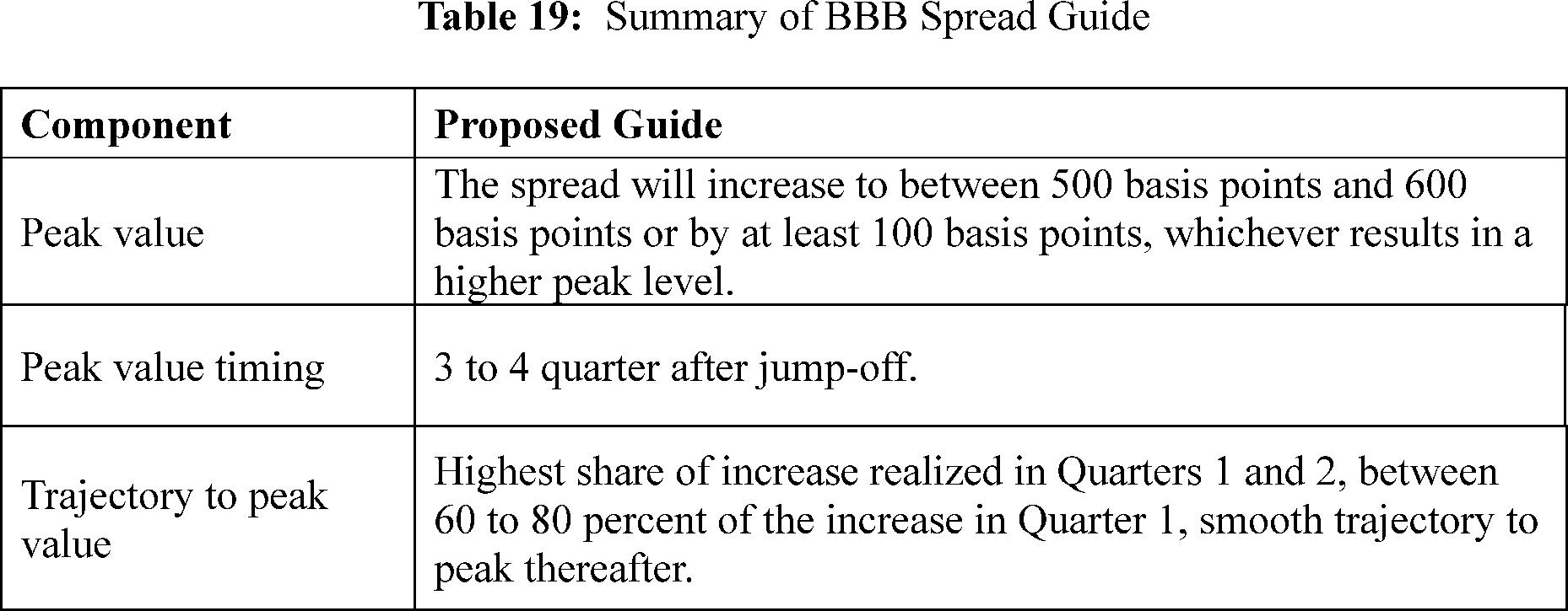

a. Peak Value Component of the Guide

The BBB corporate bond yield is expected to move such that its spread relative to the 10-year Treasury yield would either increase from its initial level by 100 basis points or to a level ranging between 500 and 600 basis points, whichever results in a higher level.

Data- and Scenario-Based Rationale for the Peak Value

In line with the guiding principles emphasized by the stress testing literature and discussed in Section IX.F of this Supplementary Information, the Board references the behavior of the BBB spreads during financial stress episodes, including the 2007-2009 financial crisis, to calibrate the guide for BBB spreads in the supervisory stress test scenarios. The higher end of the range for the peak level ( i.e., 600 basis points) corresponds to the quarterly-average peak value observed during the 2007-2009 financial crisis (Table 19). Additionally, weekly averages of the BBB spread peaked at 688 basis points over the same period.^[211] The lower end of the range for the peak level (500 basis points) is motivated by the data as well. A level of 500 basis points also constitutes a severe BBB spread value from a statistical point of view.^[212] At daily frequency, the BBB spread reached values of around 500 basis points several times during the 2007-2009 financial crisis and during the COVID-19 pandemic the BBB spread reached about 450 basis points.^[213]

These examples illustrate that the value of 500 basis points represents a severe point in the historical distribution of the BBB spread observed during crisis events, which could be followed by further worsening of conditions. Even if peaks of 500 to 600 basis points have been rather short-lived, they could potentially trigger events that would cause inadequately capitalized firms to fire-sale their assets—a risk the Board seeks to reduce through the use of stress testing. Moreover, setting a floor for the BBB spread at 500 basis points recognizes that, not only are cyclical systemic risks likely to build up at financial intermediaries during robust expansions, but that these risks are also easily obscured by a buoyant environment.

To ensure sufficient severity in the event that the BBB spread at the start of a stress test cycle is around or higher than the peak levels attained in the history ( e.g., above 500 basis points), the Board contemplates a minimum increment of 100 basis points, in line with the principle that adequate severity requires a guide to be able to go somewhat beyond historical experiences when initial conditions warrant.^[214] The minimum increment of 100 basis points ensures adequate scenario severity, maintaining the credibility of the stress test while at the same time constraining the peak from becoming unduly contractionary and deviating too far from historically observed levels.^[215] Applying a larger value of a minimum increment ( e.g., 200 basis points) could result in a peak level that is unjustifiably distant from historical peaks and might not allow the Board to reflect near-term changes, such as emerging signs of financial stabilization, resulting in inappropriately high scenario severity at a time when the economy and financial markets are already stressed.

( printed page 51915)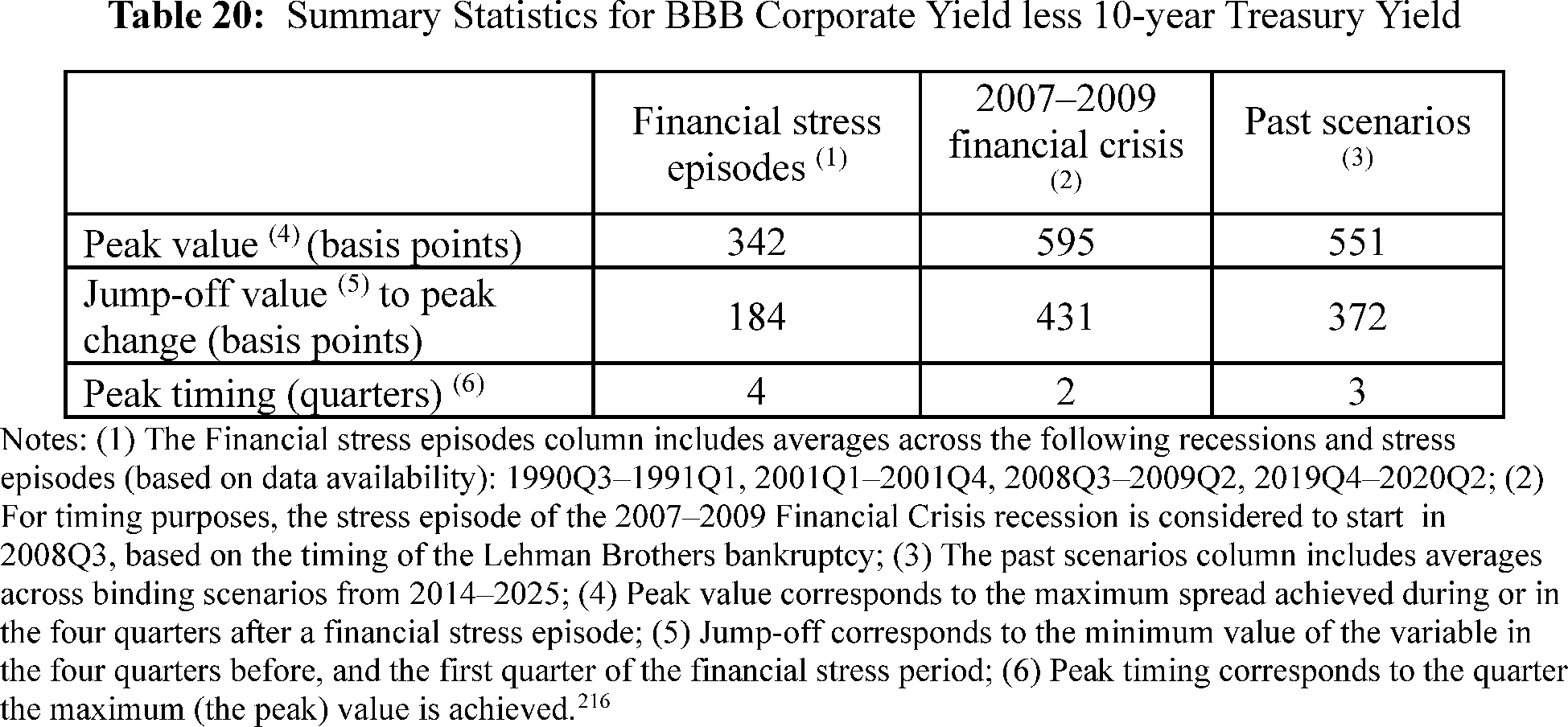

To illustrate how the Board would use this guide to formulate the scenarios, and how the implied peak levels of the guides compare to the past stress test scenarios, consider the jump-off values in 2014-2025 cycles, the period during which the Board has been conducting stress tests (Figure 6). The past stress test scenario peaks are depicted as dots in the figure, whereas the proposed guide is indicated as a range by the solid lines. This period contains both stressful times (the COVID-19 pandemic) as well as the slow recovery after 2009 and some periods of very low unemployment and robust growth. It is therefore quite representative in capturing a variety of jump-off values. In this time frame, the quarterly average of the BBB spread (depicted as a dashed line) has been between about 100 and 265 basis points at the jump-off quarter, while the average of those quarterly jump-off values was about 170 basis points. Going to 500 or 600 basis points from such jump-off values represented a substantial increase in the spread, possibly more than 400 basis points. This is a plausible increase when markets become strained or bad economic news pervades. For instance, during the 2007-2009 financial crisis, the difference between the average BBB spread during 2007Q3 and the BBB spread at the peak that episode (2008Q4) amounted to 431 basis points (Table 20).

Figure 6 also illustrates that the peak range of 500 to 600 basis points implied by the proposed guide brackets the peak values of the BBB spread used in the past stress test scenarios (the dots are located within or on the borders outlined by the solid lines throughout the time span of the figure). In other words, the proposed guide is consistent with the Board's past stress test practices in determining the peak.

( printed page 51916)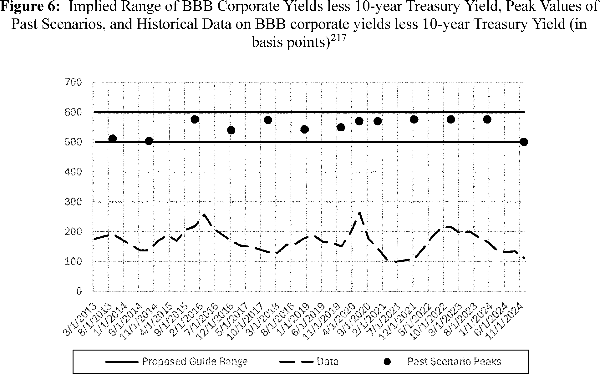

In its formulation of the annual scenarios, the Board could consider the overall level of cyclical systemic risk, or the current level of the BBB spreads as a contemporaneous indicator of uncertainty and financial stress. As discussed in Section IX.F of this Supplementary Information, the Board expects to calibrate the increment in the BBB spreads based on its views of the status of cyclical systemic risk. Specifically, the Board would be more likely to set the BBB spreads peak value at the higher end of the range if the Board expects that cyclical systemic risks are high (as it would be after a sustained long expansion), and alternatively would be more likely to set the peak value to the lower end of the range if cyclical systemic risks are low (as it would be in the earlier stages of a recovery), provided doing so remained consistent with the goal of ensuring that firms were properly capitalized to withstand severe economic and financial conditions. This might result in a scenario that is more severe than normal if the Board expects that cyclical systemic risks were increasing in a period of sustained robust expansion.

Conversely, it would also allow the Board to specify a scenario that is less severe than normal in an environment where systemic risks appeared subdued, such as in the early stages of a recovery. The lower end of the increase range could also be appropriate when underlying market uncertainty and financial stress start to recede and higher-than-usual credit losses stemming from previous elevated levels of the BBB spreads were either already realized—or are in the process of being realized—and thus removed from firms' balance sheets. This choice would consider that the scenario does not add unduly to remaining stress, thereby exacerbating the initial adverse shock, and it would be particularly appropriate if the Board judges that firms are already taking steps to reduce their risk; for instance, by potentially restricting lending to otherwise qualified borrowers.^[218]

Alternative Peak Guide Option

As an alternative, the Board also considered a guide that would choose a peak level as a maximum between 600 basis points and an increase from the jump-off value by 100 basis points. The justification for considering this peak calibration is as follows. Unlike the proposed guide, the alternative allows for less discretion and therefore would provide more certainty to firms and to market participants about the severity of the stress test each year. However, the Board considered the importance of ensuring that the chosen calibration would be sufficiently severe, because, as noted above, insufficiently severe stress tests can undermine the credibility of the results. Therefore, to attain adequate scenario severity for this option, the Board considered the peak calibration level of 600 basis points—the value corresponding to the BBB spread peak observed during the 2007-2009 financial crisis and the upper bound of the range considered for the proposed guide. This alternative guide could be less desirable as it is less flexible and may end up being too severe, especially during economic downturns, when the proposed guide would offer the flexibility to choose a lower peak from the range that could avoid adding sources of procyclicality in the results.

Consider the application of the alternative guide in 2013-2024 against the peaks of past scenarios and the proposed guide. Given the initial conditions in this time period, the alternative guide would prescribe the 600 basis points for the peak value in all quarters of the considered time span. Compared with the past stress tests, ( printed page 51917) such prescriptions are often more severe, resulting in the peaks that can be as much as 100 basis points higher than those of the past stress tests.

Although the proposed and the alternative guides are both discussed, and the Board views the alternative guide as reasonable, it was judged to be inferior to the proposed guide as discussed in this section. The purpose of the alternative guide discussion is to invite comment on a reasonable alternative considered by the Board and to transparently lay out the Board's present arguments for choosing the proposed guide.

b. Additional Guide Parameters and Rationale Behind Them

Peak Value Timing

In general, the entire 13-quarter trajectory of stress test variables is important as it ultimately affects implied firm losses. The value of the peak and its timing signify the magnitude and timing of the most severe point in this trajectory. The guide stipulates that the peak level in the scenario would be reached in quarter 3 or quarter 4, which is consistent with historical observations. In post-war recessions, the BBB spread reached its peak in quarter 4 (on average), whereas the 2007-2009 financial crisis yields a peak in quarter 2 (see Table 20). The empirical literature that studies responses of corporate spreads to shocks ( e.g., unexpected increases in uncertainty or financial riskiness) often documents a delayed peak. For instance, the response of the corporate spread to an uncertainty shock can peak after month 6 (into quarter 3) in the U.S. data.^[219] In the past stress test scenarios, the peak was also reached in quarter 4, on average.

The Board expects that the timing of the start of the stress period should sometimes differ from the start date of the recession determined by the NBER. For potentially fast-moving variables (such as BBB spread, equity prices or VIX), the Board times the onset of the stress period during the 2007-2009 Financial Crisis based on the Lehman Brothers bankruptcy on September 15, 2008. This event is widely considered to be the most significant of the events that roiled financial markets during the 2007-2009 Financial Crisis.^[220] As stress test data operate at quarterly frequency, the Board's timing of this event for purposes of dating the peak of the BBB corporate spread is in 2008Q3. Indeed, the BBB corporate spread remained largely flat between 2008Q1 and 2008Q2, rising somewhat in 2008Q3 (because the Lehman Brothers bankruptcy occurred close to the end of the quarter, it had little effect on the quarterly average) before increasing sharply to the observed maximum in 2008Q4.^[221] Therefore, the focus on the Lehman Bankruptcy as the triggering event is more consistent with the stress test scenario narrative in which a financial shock sets the stress test scenario dynamics in motion than the NBER recession date.

Trajectory to Peak Value

To reach the peak spread value, the guide prescribes that the highest share of the spread increase (about 60 to 80 percent) occurs in the first quarter of the scenario. Such frontloading of the spread increase is consistent with the historical evidence and academic literature.^[222] For instance, in the 2007-2009 financial crisis, the largest increase in the spread (about 67 percent of the jump-off. A very similar result emerges when considering the Enron/Dotcom stress episode and 1990 bond market stress episode.^[223] On average (across all three bond market stress episodes), about 66 percent of the increase to the peak in the spread was realized in a single quarter after the onset of the stress episode. After quarter one and until the peak is reached, the guide stipulates a smooth trajectory with half of the remaining adjustment made in quarter two and with the rest of the adjustment made either in quarter three (when the peak occurs in quarter three) or equally distributed between quarter three and four (when the peak occurs in quarter four). As an example, if the increase share in the first quarter was around 60 percent, then the adjustment in quarter two would be about 20 percent with the remaining 20 percent in quarter three (if the peak is in quarter three) or with the remaining distributed approximately 10 percent each in quarter three and four (if the peak is in quarter four). This simple adjustment rule mimics a hump-shaped response of the corporate spread to shocks, a feature well-documented in the empirical literature.^[224]

Mortgage Rate

The stress test scenarios sets out trajectories for several variables, including the mortgage spread as proxied by the quarterly average of weekly series for the interest rate of a conventional, conforming, 30-year fixed-rate mortgage, obtained from the Freddie Mac Primary Mortgage Market Survey relative to the 10-year Treasury yield.^[225] For purposes of this guide, mortgage spread refers to the difference, in basis points, between mortgage and Treasury rates defined above.

In the supervisory stress test, the mortgage spread can act as both (i) an indicator of stress for certain important assets under the scenarios and (ii) a source of stress for firms subject to the supervisory stress test with substantial exposure to assets that are tied to mortgage spreads, such as mortgage loan portfolio or mortgage-backed securities, which are reported by firms on FR Y-14M, Schedule A (First Lien) and FR Y-14Q, Schedule B (Securities). Firms subject to the supervisory stress test typically have substantial exposure to the assets referenced in the mortgage spread, and as a result, by incorporating the mortgage spread into scenarios, stress tests help ensure that firms are prepared for a wide range of market conditions, including periods of ( printed page 51918) elevated mortgage spreads, in part reflecting financial shocks and any associated economic downturn. This helps maintain the overall stability and resilience of the financial system.

The Board uses a quarterly average of the mortgage rate spread in the stress test scenarios. Quarterly averages smooth out excessive (and potentially irrelevant) volatility that is present at weekly or monthly frequencies. Using quarterly averages strikes a balance between being sensitive enough to capture market trends and stable enough to avoid overreaction to market volatility that is not representative of underlying trends in housing markets or the broader economy.

In determining the appropriate level of scenario severity, the Board adheres to scenario design principles discussed in Section IX.F of this Supplementary Information. While doing so, the Board also strives to avoid introducing additional sources of procyclicality into the financial system. In the context of the mortgage spread, these principles are applied in calibrating three key aspects of the guide: the trough value, the timing of the trough value, and the trajectory to trough. This approach helps ensure that the mortgage spread guide aligns with the established stress testing literature while mitigating potential systemic risks for the financial system.

The rest of this section is organized as follows. First, Table 21 provides an overview of the mortgage rate guide components, which is followed by a description of the peak component for the guide. The next subsection provides the data- and scenario-based rationale for the calibration of the peak component. A discussion of an alternative peak option follows in the next section, comparing the implementation and caveats to the proposed guide option. Finally, additional guide parameters (trough value timing and trajectory to the peak) and the rationale for their calibration are discussed.

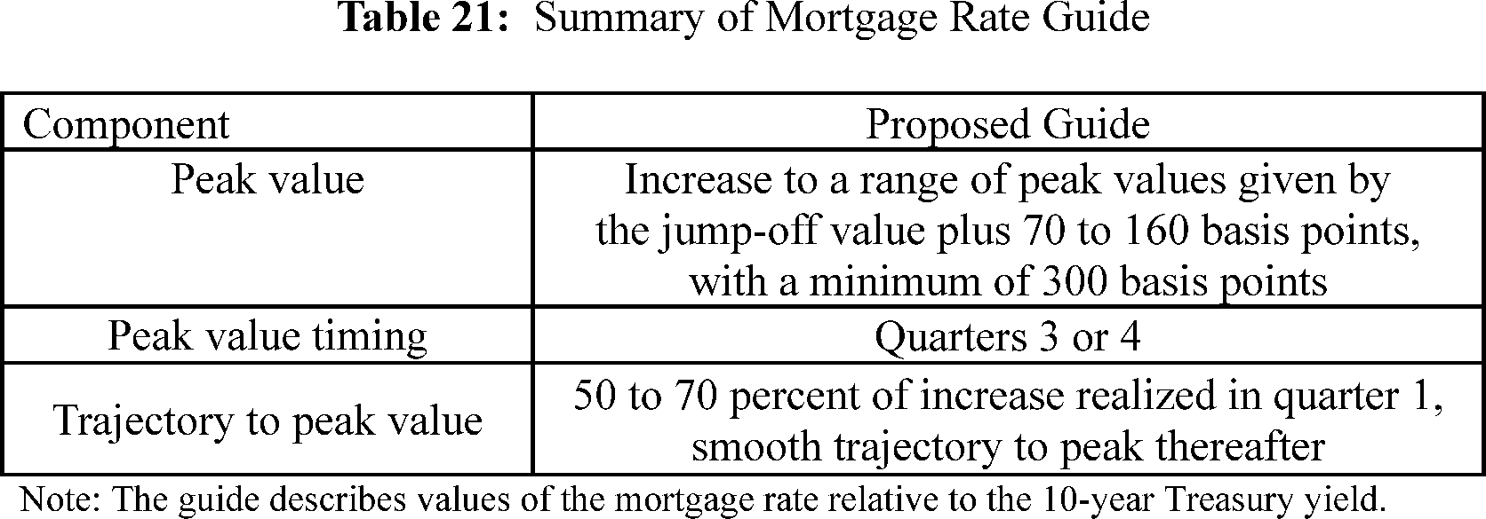
a. Peak Value Component of the Guide

The mortgage rate is expected to move such that its spread relative to the 10-year Treasury yield would increase from its jump-off level ( i.e., the value of the variable in the quarter before the start of the scenario) to a range determined by that level plus 70 basis points to 160 basis points, with a lower bound of 300 basis points.

Data- and Scenario-Based Rationale for the Peak Value

In line with the guiding principles emphasized by the stress testing literature and discussed in Section IX.F of this Supplementary Information, the Board uses the behavior of the mortgage spreads during financial stress episodes, including the 2007-2009 financial crisis, to calibrate the guide for the mortgage spread in the supervisory stress test scenarios. In particular, the Board considers the behavior of the mortgage spread in three severe recessions, including the 2007-2009 financial crisis, to calibrate the guide for mortgage spreads in the supervisory stress test scenarios. In particular, the calibration of the lower bound of 300 basis points in the guide is based on evidence from historical stress episodes along with the principle of conservatism. The average peak value for the mortgage spread observed in severe recessions has been 278 basis points (Table 22), ranging from 225 to 380 basis points.^[226] In the 2007-2009 financial crisis, the peak mortgage spread measured about 249 basis points at a weekly frequency.^[227] The calibration of the lower bound of 300 basis points—a value that is slightly above the historical average during severe recessions—speaks to the guiding principle that adequate severity should be somewhat beyond historical experiences. In addition, setting a floor for the mortgage spreads at 300 basis points recognizes the fact that, not only do cyclical systemic risks build up at financial intermediaries during robust expansions, but that these risks are also easily obscured by a buoyant environment.

( printed page 51919)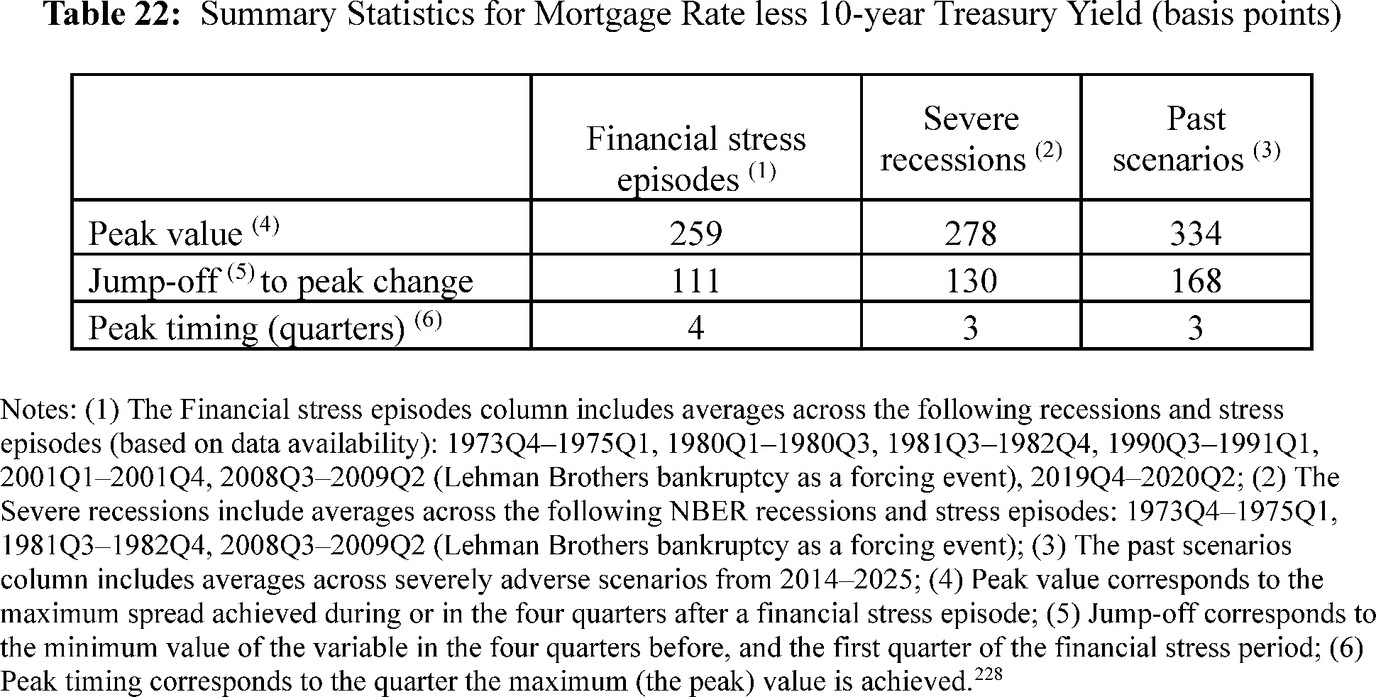

The historical ^[228] maximum value of the mortgage spread occurred in the 1980-1985 episode—in a high-inflation environment with high unemployment as well—and measured 404 basis points, based on quarterly averages of the spread. Weekly averages of the spread during this episode would result in a higher peak level of 541 basis points, which was reached in the calendar week ending on April 20, 1980 (Figure 7). Between 2022 and 2024, inflation accelerated, and the mortgage spread rose above the 2007-2009 peak, reaching a quarterly-frequency maximum of 284 basis points in 2023 Q2 (304 basis points at a weekly frequency, in the calendar week ending on May 28, 2023) despite a strong economy and well-functioning mortgage markets. Hence, guide calibration of the mortgage spread should account for conditions in the housing market, including interest rate volatility, and the phase of the business cycle as described above, as well as the level of inflation and inflation expectations at the jump-off quarter to elucidate their effect on firms' balance sheets.

( printed page 51920)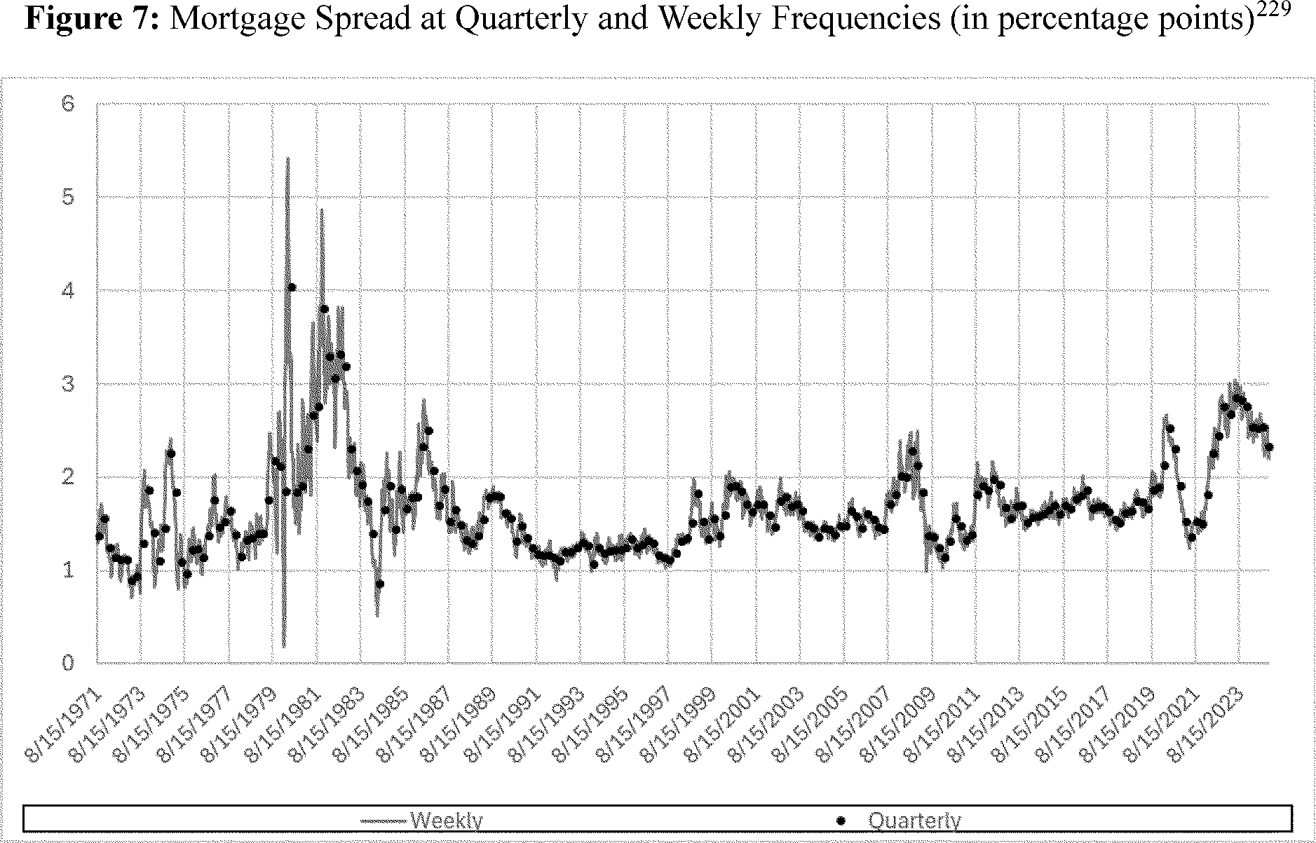

In its formulation ^[229] of the annual scenarios, the Board could consider the overall level of cyclical systemic risk, or the current level of the mortgage spreads as a contemporaneous indicator of uncertainty and financial stress. As discussed in Section IX.F of this Supplementary Information, the Board expects to calibrate the increment in the mortgage spreads based on its views of the status of cyclical systemic risk. Specifically, the Board would be more likely to set the mortgage spread peak value at the higher end of the range if the Board expects that cyclical systemic risks are high (as it would be after a sustained long expansion), and alternatively would be more likely to set the peak value to the lower end of the range if cyclical systemic risks are low (as it would be in the earlier stages of a recovery), provided doing so remained consistent with the goal of ensuring that firms were properly capitalized to withstand severe economic and financial conditions. This might result in a scenario that is more intense than normal if the Board expects that cyclical systemic risks were increasing in a period of sustained robust expansion. Conversely, it would also allow the Board to specify a scenario that is less intense than normal in an environment where systemic risks appeared subdued, such as in the early stages of a recovery. The lower end of the range could also be appropriate when underlying market uncertainty and financial stress start to recede and higher-than-usual credit losses stemming from previously elevated levels of mortgage spreads were either already realized or are in the process of being realized, and thus removed from firms' balance sheets. This choice would consider that the scenario does not add unduly to remaining stress, thereby exacerbating the initial adverse shock, and it would be particularly appropriate if the Board judges that firms are already taking steps to reduce their risk—for instance, by potentially restricting lending to otherwise qualified borrowers.^[230]

Consider the application of the range component of the guide (70 to 160 basis points from the jump-off value) illustrated in Figure 8 (solid lines) for 2014-2025 stress test cycles. This time period is illustrative as it contains various stages of the business and financial cycle (normalization after the 2007-2009 financial crisis, the COVID-19 pandemic and the normalization after it in a higher-inflation environment). Accordingly, the initial conditions in this period are quite representative. While the lower bound of the range (300 basis points) was explained above, the application of the upper part of the range results in values from 300 basis points to 440 basis points, with the higher values achieved in 2022-2024, a period of higher inflation. Per the discussion above, these values, while being severe, do not deviate too far from historically observed values. And consistently with historical experiences, these values also reflect the inflation environment.

( printed page 51921)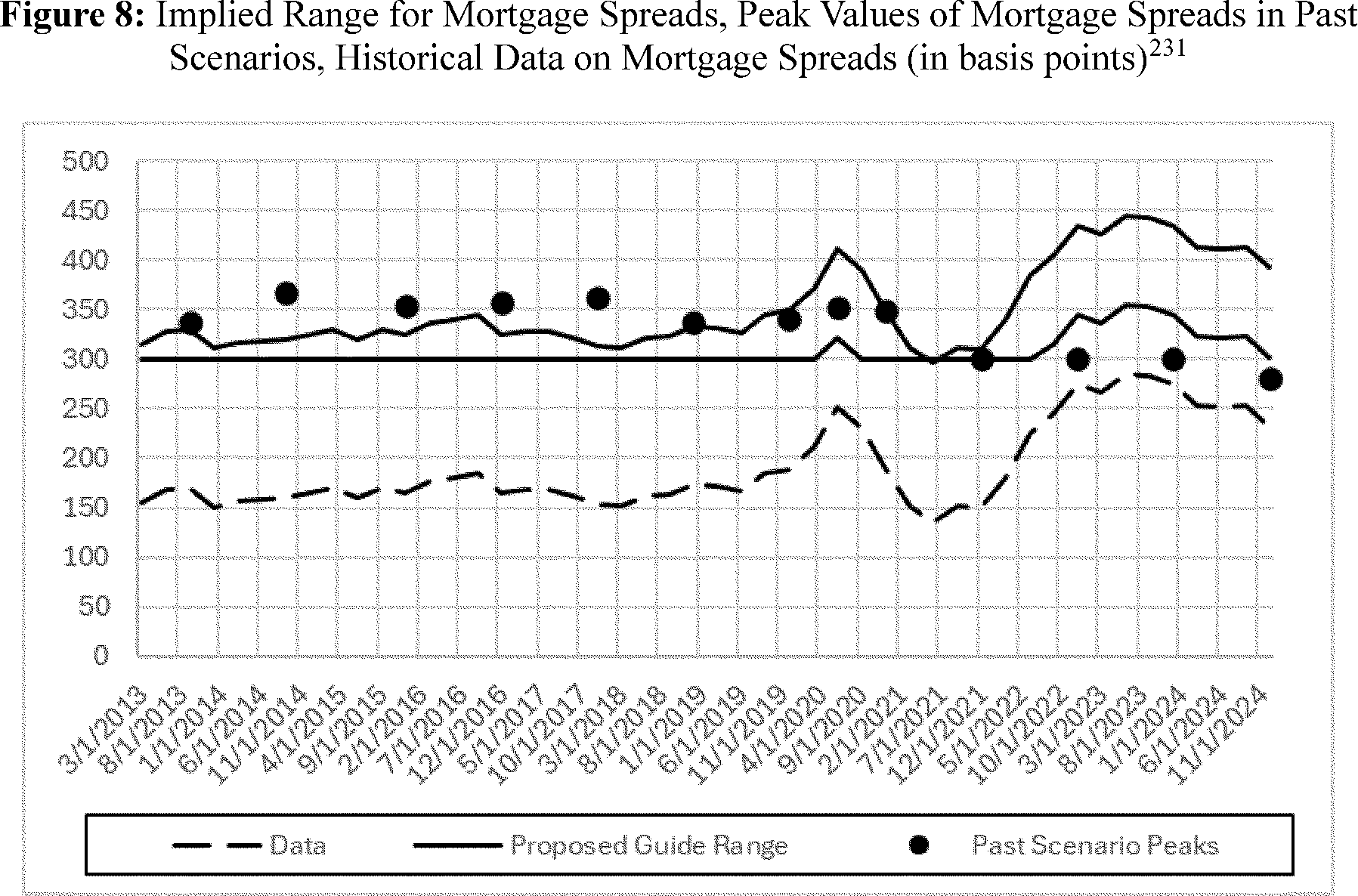

To illustrate ^[231] the implications of the guide, the Board applies it to recent historical data and compares the implied peak prescriptions with the corresponding peaks from past stress test scenarios (Figure 8). From 2013Q1 until 2019Q4, the stress test peak values, depicted by the dots, were quantitatively close to the upper end of the range of the proposed guide, depicted by the solid lines (Figure 8). From the onset of the COVID-19 pandemic in 2020 through 2021, the stress test peaks were mostly within the bands of the proposed guide, while in 2022-2024 the stress test peaks were located at or very close to the lower end of the range suggested by the proposed guide. Summing up, comparison of the guide-implied peaks with the past stress test peak values shows that the guide is broadly consistent with past scenario values. The range of the guide should allow the Board to account for risks that are apparent in relevant indicators of economic and financial conditions and constrain the peak to historically plausible bounds during normal periods, while adjusting to future periods in which spreads may move toward record levels.

Alternative Peak Guide Option

As an alternative, the Board also considered a guide that would choose a peak level as a maximum between 300 basis points and an increase from the jump-off value by 100 basis points. A comparison of the alternative and the proposed guides in 2013-2024 illustrates episodes when the alternative guide deviates from the proposed guide. As the alternative guide has a flat increment regardless of the underlying conditions, it would propose systematically lower peak values in the pre-pandemic period and systematically higher values in the post-pandemic period, when compared with the stress test peaks. Additionally, following this alternative guide would not allow the Board to respond to risks not already reflected in the current level of the mortgage spread.

Although the proposed and the alternative guides are both discussed, and the Board views the alternative guide as reasonable, the benefits to the public from increased predictability in the alternative guide are considered to be outweighed by the added flexibility to reflect risks related to mortgage finance that are apparent in relevant indicators of economic and financial conditions or to avoid adding additional sources of procyclicality in the proposed guide. The purpose of the alternative guide discussion is to invite comment on a reasonable alternative considered by the Board and to transparently lay out the Board's present decision making in choosing the proposed guide.

b. Additional Guide Parameters and Rationale Behind Them

Peak Value Timing

In general, the entire 13-quarter trajectory of stress test variables is important as it ultimately affects implied firm losses. The value of the peak and its timing signify the magnitude and timing of the most severe point in this trajectory. The proposed guide stipulates that the peak level in the scenario would be reached in quarters 3 to 4, which is consistent with historical observations and past severely adverse scenarios (Table 22). The proposed guide sets a range of peak timings between 3 and 4 quarters, whereas the alternative guide eliminates this flexibility and stipulates a peak in quarter 3. Keeping the magnitude of the peak constant, a more delayed peak timing generally results in less severity of the overall path, as a less abrupt worsening in conditions and credit quality gives firms and mortgage borrowers more time to adjust to the shock. In contrast, an earlier peak timing would increase the scenario severity.

For the proposed guide, a range in the timing (quarter 3 or quarter 4) is used as an additional lever (together with the peak magnitude range) to avoid adding ( printed page 51922) sources of procyclicality in the stress test. An earlier peak timing would increase the scenario severity. The factors that the Board would consider in setting the timing of the peak are the same as those discussed above influencing the level of the peak.

Trajectory to Peak Value

To reach the peak spread value, the guide prescribes that the highest share of the spread increase (50 to 70 percent) occurs in the first quarter of the scenario. After quarter one and until the peak is reached, the guide stipulates a smooth trajectory. Such frontloading of the spread increase is consistent with the historical evidence and academic literature.^[232] Averaging across all financial stress episodes, the share of the mortgage spread increase that occurs in the first quarter after the onset of the stress is about 60 percent; in other words, 60 percent of the distance from the jump-off point to the peak is covered in the first quarter. This number is quantitatively similar to the past stress test scenarios in 2013-2025, where on average the corresponding share measures 64 percent. Averaging across severe historical episodes in the data yields a share of 73 percent. At the same time, there are severe episodes with a somewhat smaller increase in the share occurring in the first quarter. For instance, the severe episode surrounding the 1981 recession measured 47 percent of the mortgage spread increase in the first quarter. Hence, both the guide calibration (over 50 percent) as well as the average obtained across the mortgage spread paths in 2013-2025 stress test scenarios (64 percent) lie within historically plausible bounds.

International Variables

As described in the Scenario Design Policy Statement, a scenario that targets all specific risk factor groups includes judgement on the projected paths of selected international variables. Recessions that occur simultaneously across countries are an important source of stress to the balance sheets of firms with notable international exposures but are not a typical feature of the international economy even when the United States is in recession. As a result, simply adopting the typical path of international variables in a severe U.S. recession would likely underestimate the risks stemming from the international economy. Consequently, an approach that relies on both judgement and insights from economic models informs the path of international variables. As part of the review of the scenario design framework, the Board has developed simple quantitative guides for the proposed paths of the international variables used in the severely adverse scenario of the supervisory stress test. Consistent with the Scenario Design Policy Statement, the international component of the stress test scenarios contains the path for real GDP, consumer price inflation, and the nominal exchange rate for four country blocs: the euro area, the U.K., Japan, and Developing Asia.^[233] These economies capture the majority of the foreign exposure of U.S. banks.

The following guides apply to each international variable:

• Apeak/trough value, which represents the extreme value (either peak or trough, depending on the variable) that is typically reached in the severely adverse scenario. For all variables the peak/trough is reached after 4 quarters.
• Anend value for the last period in the scenario, that is 13 quarters after initial impact.
• A scenariopath, which describes the path of international variables from the jump-off value to the peak/trough value and then to the end value.
• A scenariorange, which specifies by how much each variable can deviate from the scenario path to adapt to relevant changes in banking, macroeconomic, or other conditions.

a. Overview of Approach

In designing the paths of the international variables in the severely adverse scenario, the Board opted to follow a prescriptive approach that is informed by the experience of the 2007-2009 financial crisis. Given its global repercussions, the 2007-2009 financial crisis is a useful benchmark for the economic effects of a large global financial shock.

To generate the proposed paths of GDP and inflation in the four economic regions for the severely adverse scenario, the Board first computed the distance between the realized outcomes of GDP and inflation during the 2007-2009 financial crisis from the baseline forecasts prior to the onset of the 2007-2009 financial crisis. These baseline forecasts were derived from publicly available forecasts from the Blue Chip Economic Indicators and the IMF World Economic Outlook (WEO).^[234] The Blue Chip and WEO forecasts provide values for year-over-year real GDP growth and inflation. To forecast quarterly GDP growth rates and inflation rates, quarterly values are first derived from the annual growth rates using linear interpolation; then a Hodrick-Prescott filter is used to smooth the path of GDP and inflation across the forecast period.^[235] Based on this procedure, the Board specifies guides for the values of the variables of interest. These values are usually reached in the scenario, but the Board reserves the right to depart from these values within specified ranges.

The data for the euro area, the U.K., and Japan were aggregated to obtain identical guides for GDP and inflation for these Advanced Foreign Economies (AFEs). The Board favored identical guides for these regions to prevent possible credit allocation incentives that could arise if guides differed systematically between the AFEs. However, identical guides do not imply that the actual severely adverse scenario features identical paths for the euro area, the U.K., and Japan. The scenario paths of the three regions can vary with the given ranges.

The key elements of the international guides derived from this procedure are summarized in Table 23; Figure 9 shows the behavior of the variables of interest during the 2007-2009 financial crisis from which the guides are derived. Detailed explanations and alternative considerations are provided thereafter. For GDP, the deviation is computed as percentage change from the baseline real GDP level. For inflation, the deviation is computed as percentage point difference from the baseline path of inflation. For exchange rates, the guide is expressed in terms of percent deviation from the jump-off point.

( printed page 51923)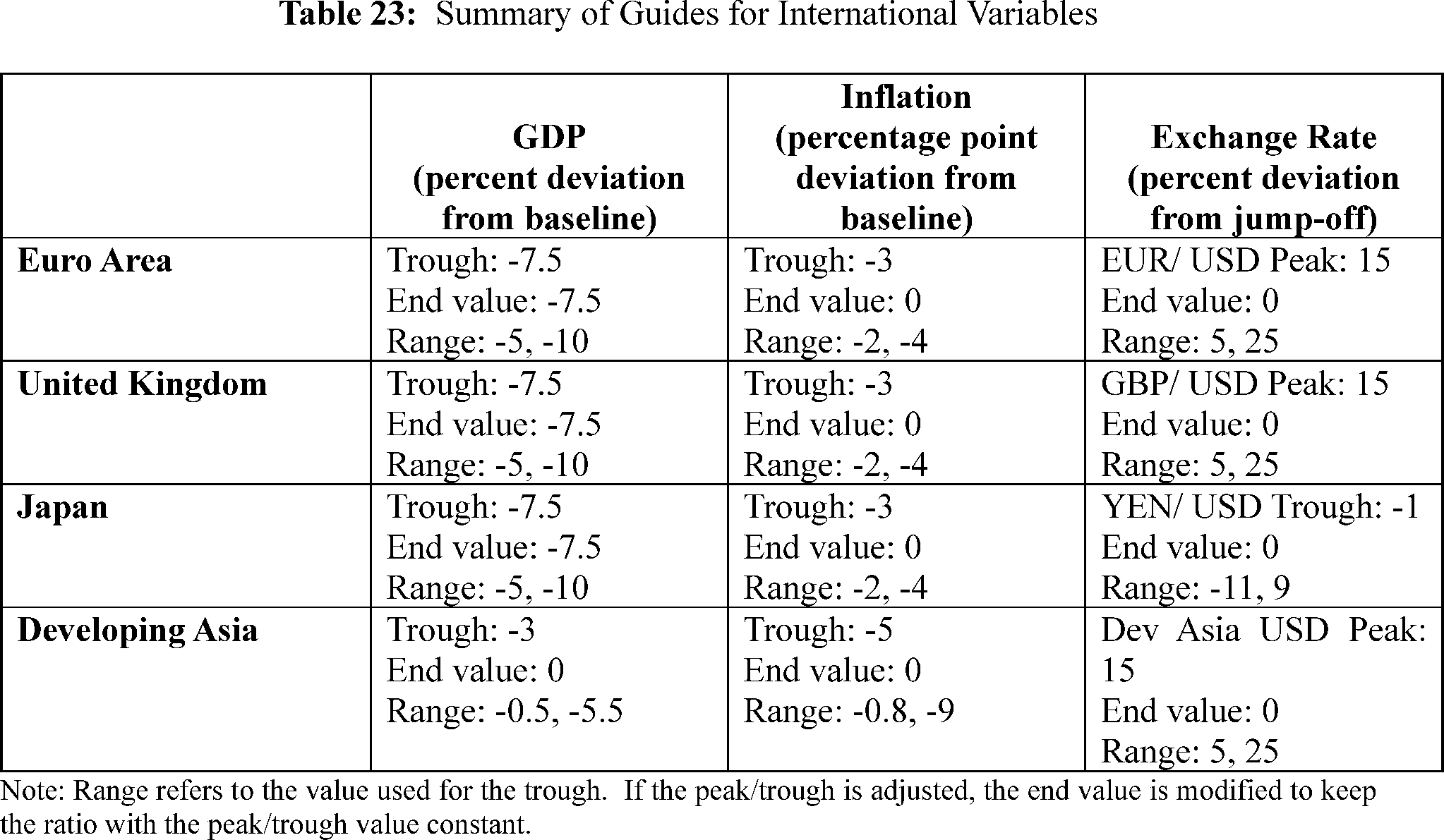

Table 23 also provides ranges for each variable to allow for flexibility: This flexibility enables judgment to be exercised to capture the possibility that the foreign economies might react differently to financial stress, either because of changes in the global macroeconomic landscape or in country-specific vulnerabilities.

The prescriptive approach for the international variables in the severely adverse scenario yields guides that are qualitatively and quantitatively reasonable based on the Board's judgment and broadly accepted models of international economies.^[236] The Board opted for the more prescriptive approach because the advantages of increased transparency and simplicity outweighed the disadvantage of less flexibility.

b. GDP

Trough Value

The magnitude of the prescribed economic downturn in the specified foreign economies is informed by the deterioration in foreign economic activity which occurred between 2008Q1 and 2009Q1. In particular, the trough value for GDP is obtained by considering the deviation of the real GDP level in 2009Q1 from a baseline path derived from the April 2008 IMF WEO forecast.^[237] This approach implies that, four quarters after jump-off, the GDP levels in the euro area, the U.K., and Japan are 7.5 percent below the baseline scenario.^[238] In Developing Asia, GDP growth declines until GDP reaches a level 3 percent below baseline. These values are in line with the behavior of real GDP reported in the top panel of Figure 9.

End Value

In the euro area, the U.K., and Japan, the level of GDP at the end of the severely adverse scenario deviates from the corresponding value in the baseline (13 quarters after initial impact) by the same magnitude as the trough value of GDP deviates from the corresponding value in the baseline (4 quarters after initial impact). This assumption implies that, in line with the experience of the 2007-2009 global financial crisis, after reaching the trough, GDP in the AFEs grows at the same rate as in the (pre-crisis) baseline. The guide proposes that GDP recovers more quickly in developing Asia, returning to the GDP baseline in levels at the end of the scenario, in line with the evidence from 2011Q2. These GDP paths are consistent with Figure 9 and with empirical evidence which suggests that advanced economies suffer very persistent output losses following a financial crisis, while developing economies experience less severe slowdowns.^[239]

Path

Real GDP reaches the reference trough four quarters after the jump-off date and then gradually converges to the end value of the scenario. After reaching the trough, the AFEs experience a similar GDP growth rate in the scenario as in the baseline, whereas Developing Asia grows faster in the scenario to catch up with the level of GDP in the baseline. The path of GDP is created with a two-step procedure similar to the one used to generate the baseline scenario. First, the series is linearly interpolated between the jump-off value and the ( printed page 51924) trough value and from the trough value to the end value. Then, a Hodrick-Prescott filter is used to smooth the GDP path over the duration of the scenario. This approach generates a smooth path for GDP consistent with business cycle dynamics.

Range

The path described above captures the GDP dynamics during the 2007-2009 financial crisis. In determining the magnitude of the international shock in the severely adverse scenario, the Board would consider several factors, including the current economic performance of foreign economies, the risks posed by country-specific vulnerabilities, and the scope for countercyclical policy actions in each country bloc. For example, in periods of sub-par foreign economic performance, the Board would likely reduce the magnitude of the shock, whereas when foreign growth is particularly strong, the magnitude of the shock would be increased. In addition, the allocation of shocks across blocs can be altered to highlight relevant country-specific risks. This strategy is implemented by increasing or decreasing the severity of the shock, as measured by the deviation of GDP from baseline at the scenario trough, by at most 2.5 percent.^[240] As a result, at the trough, real GDP can fall between 5 and 10 percent below the baseline in advanced foreign economies, bracketing the real GDP outcomes of the three AFEs in the 2007-2009 financial crisis. For Developing Asia, real GDP can fall between 0.5 and 5.5 percent below the baseline. These adjustments are performed while keeping the overall stress on foreign economies, as measured by the average GDP deviation from baseline at the trough, within a range of 4 to 9 percent.^[241]

( printed page 51925)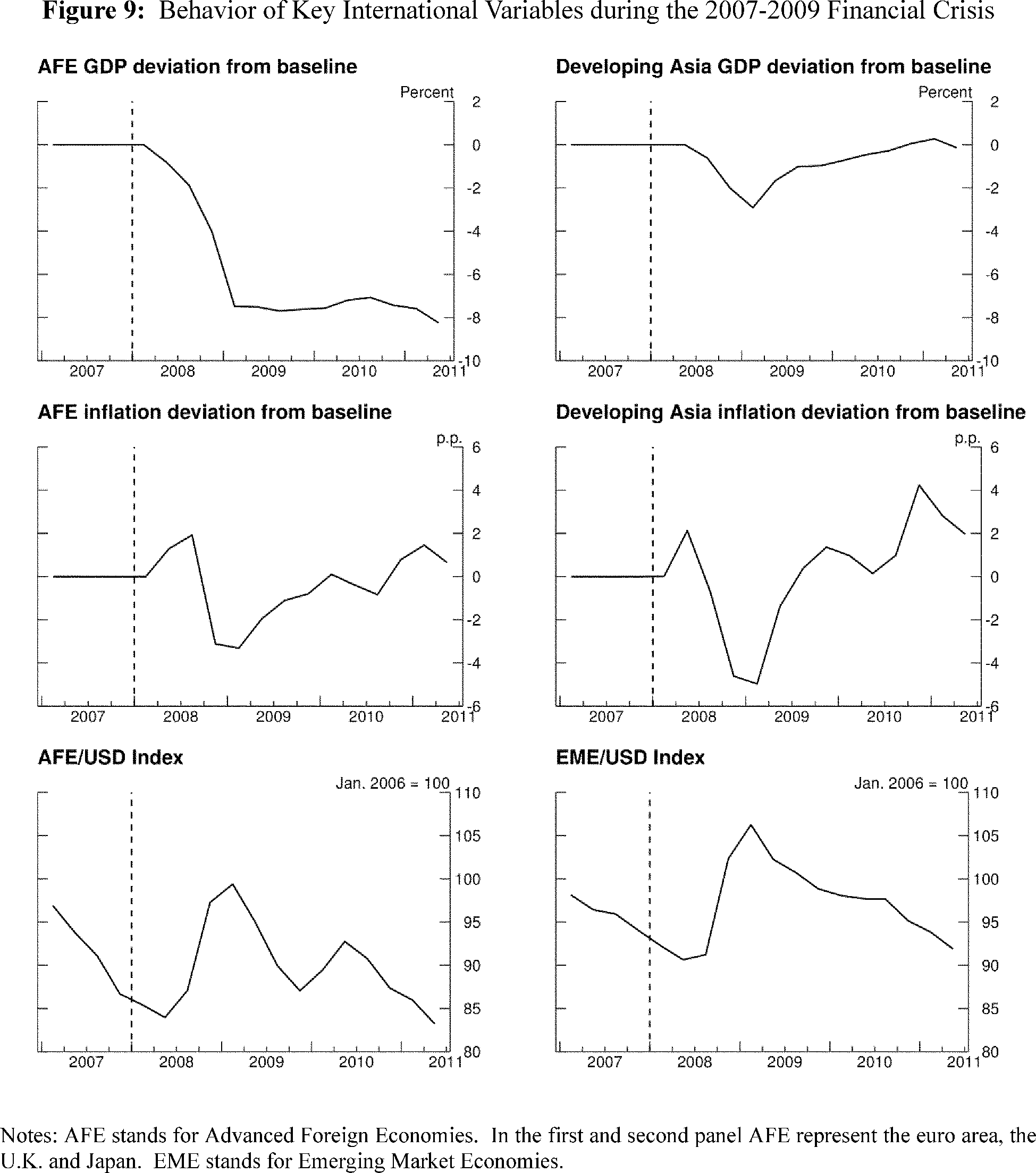

c. Inflation

Trough Value

Inflation is assumed to decline below the baseline scenario for the first four quarters of the simulation, consistent with the demand-driven decline in GDP growth over the same period. This behavior is broadly in line with the historical evidence between 2008Q1 and 2009Q1 for the four country blocs. The maximum decline in inflation is calibrated to reflect the difference between the realized rate of inflation and the one derived from the April 2008 IMF WEO forecast for 2009Q1 (middle panel of Figure 9Figure). This method provides that, four quarters after the jump-off date, inflation is below baseline by about 3 percentage points in the euro area, the UK, and in Japan, and by 5 percentage points in Developing Asia.^[242]

End Value

After reaching the trough, inflation gradually returns to baseline by the 13th quarter of the simulation. This inflation path is consistent with the evidence from the 2007-2009 financial crisis, when inflation returned to, or even surpassed, the WEO baseline by 2011. In ( printed page 51926) addition, academic research suggests that financial crises typically do not have large or persistent effects on inflation.^[243]

Path

The path for inflation is obtained by using the same strategy employed for GDP, which combines linear interpolation and a Hodrick-Prescott filter.

Range

If the path of GDP is different from the reference path, the path for inflation will be adjusted to preserve the same ratio between the deviation of GDP and the deviation of inflation from baseline under the reference path—the values of these ratios are 2.5 for advanced foreign economies and 0.6 for Developing Asia.^[244] As a result, inflation declines between 2 percentage points and 4 percentage points below baseline in the advanced foreign economies, and between 0.8 percentage points and 9 percentage points below baseline in Developing Asia.

d. Exchange Rates

Trough/Peak Value

The Board assumes that over the first four quarters of the simulation the U.S. Dollar experiences a 15 percent appreciation against the Euro and the British Pound. This appreciation is in line with the change in the Nominal Advanced Foreign Economies U.S. Dollar Index between 2008Q1 and 2009Q1 (bottom left panel of Figure 9).^[245] Over the same period, the U.S. Dollar appreciates by 15 percent also against the exchange rate for Developing Asia, in line with the fluctuation in the Nominal Emerging Market Economies U.S. Dollar Index between 2008Q1 and 2009Q1 (see bottom right panel of Figure 9).^[246] Consistent with the evidence between 2008Q1 and 2009Q1, the U.S. Dollar experiences a mild 1 percent depreciation against the Japanese Yen, which is typically considered a safe-haven currency, a currency which retains its value during times of global economic stress.^[247]

End Value

Exchange rates gradually reach their peak/trough and then revert back to their jump-off values by the end of the scenario horizon.

Path

The path for the exchange rate is obtained by using the same strategy employed for GDP and inflation, which combines linear interpolation and a Hodrick-Prescott filter.

Range

For exchange rates, which are highly volatile and only weakly linked to macroeconomic fundamentals, the Board can adjust the maximum fluctuation of each of the four foreign currencies within a range of plus or minus 10 percent from the reference peak/trough value.^[248] For each country bloc, the magnitude of the depreciation is adjusted depending on the realized change in the exchange rate in the year preceding the jump-off date. For example, if over the past year the dollar has already appreciated by 5 percent against the euro, the Board would lower the appreciation rate in the scenario from 15 percent to 10 percent.

e. Alternative Considerations

The Board considered a range of different approaches to derive the guides for the international variables in the severely adverse scenario. First, distinct instead of common guides for GDP and inflation for each of the AFEs were explored. Following the methodology explained in Section IX.F of this Supplementary Information, the trough values for GDP during the 2007-2009 financial crisis were 6 percent below baseline in both the euro area and the U.K., and 10 percent below baseline in Japan. For inflation, the trough values in the 2007-2009 financial crisis were 3 percent below baseline in the euro area, 2 percent below baseline in the U.K., and 4.5 percent below baseline in Japan. The Board decided against using region-specific guides for the AFEs, as systematic differences in the guides across regions could affect credit allocations. However, the issued guides still allow for region-specific paths in the severely adverse scenario within the specified ranges to reflect region-specific circumstances when desirable. The Board may also use the specified ranges to raise or lower the sensitivity of all regions at the same time in the severely adverse scenario.

Second, the Board examined other global or regional economic downturns of significance in addition to the 2007-2009 financial crisis to refine its guides for the international variables of the adverse scenario. There are only a few global recessions in recent history but none of them—besides the 2007-2009 crisis—were driven by financial factors. The COVID-19 recession of 2020 led to a sharper contraction in global economic activity than the 2007-2009 financial crisis but did not result in persistent financial stress. One distinct feature of the 2007-2009 financial crisis was the resilience of Developing Asia where GDP dropped by only 3 percent relative to baseline. Only a decade prior to the 2007-2009 financial crisis, several countries in Developing Asia had experienced negative doubled-digit GDP growth rates as part of the 1997 Asian Financial Crisis. Based on the experience of the 1997 Asian Financial Crisis, the Board considered a lower trough value for Developing Asia. However, the Board decided against this approach for several reasons. China was generally unaffected by the Asian Financial Crisis and maintained its high GDP growth rate throughout the crisis, significantly increasing the regional GDP growth rate during this period despite the sharp declines experienced elsewhere in the region. In addition, the countries that were most affected by the Asian Financial Crisis changed to more robust economic policies—switching from fixed/managed exchange rates to flexible inflation targeting and from policies that implied large current account deficits to policies that led to surpluses. Finally, the Board looked to the euro area debt crisis for additional guidance. But since this crisis directly followed the 2007-2009 financial crisis no additional insight for the design of the severely adverse scenario was obtained that was not already embedded in the analysis of the 2007-2009 financial crisis. In the interest of transparency and simplicity, the Board decided to adopt the findings derived solely from the 2007-2009 financial crisis but added flexibility by allowing ranges for variables. ( printed page 51927)

H. Global Market Shock

Design of the Global Market Shock

The global market shock component comprises a large set of financial risk factors and associated hypothetical shocks to those risk factors. The Board considers emerging and ongoing areas of financial market vulnerabilities in the development of the global market shock component, informed by financial stability reports, supervisory information, and internal and external assessments of potential sources of distress such as geopolitical, economic, and financial market events. Financial risk factor shocks are calibrated based on assumed time horizons that reflect several scenario design considerations. The Board also considers liquidity characteristics of the different asset classes that constitute certain risk factors. These liquidity horizons approximate the variation in speed at which banks could reasonably close out, or effectively hedge, the associated risk exposures in the event of market stress.

The chosen risk factors of the global market shock scenario are important to specifying how a stress scenario unfolds across financial markets and capturing salient risks within the banking system. These include, but are not limited to:

• Public equity returns from key advanced economies and from developing and emerging market economies, along with selected points along term structures of equity option-implied volatilities;
• Exchange rates of foreign currencies, along with selected points along term structures of foreign exchange option-implied volatilities;
• Government yields at selected maturities (e.g., 10-year U.S. Treasuries), swap rates, and other types of interest rates for key advanced economies and from developing and emerging market economies;
• Implied volatilities on interest rate options for selected maturities and expiration dates, which are key inputs to the pricing of interest rate derivatives;
• Futures prices at various expiration dates for commodity products such as energy, oil, metals, and agricultural products; and
• Credit spreads or prices for selected credit-sensitive products, including corporate bonds, credit default swaps (CDS), securitized products, sovereign debt, and municipal bonds.

The global market shock is typically applied to positions held by the firms on a given as-of date, reflecting a hypothetical instantaneous “shock” to a large number of risk factors that determine the mark-to-market values of trading positions. Additionally, the global market shock in a given annual severely adverse scenario is a standardized set of market shocks that apply to all of the firms with significant trading activities. The selection of a single date, and a single global market shock, has tended to enhance the operational consistency and simplicity of the annual supervisory stress test, while managing burden on reporting firms.

The Board is considering enhancements to the design of the global market shock in the annual stress test to improve the stress test's ability to capture the impact of severe economic stress in financial markets. Alternative approaches to the global market shock could include employing instantaneous shock events across multiple as-of dates, rather than the current approach of selecting a single date for an instantaneous shock event. Another approach could involve an annual stress test that features multiple global market shock components on a single as-of date, which would allow the Board to compare a given firm's losses across a variety of types of shocks for a given set of trading position. The set of losses generated by such multiple market scenarios could be aggregated using a simple average, an average of the two worst outcomes, or another technique. These alternatives could enhance the dynamism of the annual stress tests and improve the Board's ability to evaluate the impact of severe economic stress on trading positions in a given annual stress test. However, these changes could also increase the complexity of the tests, and affect their predictability from year to year.

Question 44: What changes could the Board implement to improve the general design of the global market shock? What, if any, alternative approaches should the Board consider? For instance, should the Board consider adjusting the global market shock so that shock events occur on multiple dates within the as-of date window? Should the Board consider testing more than one global market shock component in a given annual stress test or on a particular date? If so, how should the Board assess whether the current design, or alternative approaches, contribute to outcomes that are overly volatile or insufficiently representative of risks? If the Board should adopt these alternative approaches, what information should the Board provide to the public about how it will implement these alternatives, and should that information be published as part of a revised Scenario Design Policy Statement, codified as part of Regulation YY, the annual scenario disclosure, or some other means?

Question 45: If the Board did adjust the global market shock to consider multiple dates within the as-of date window or more than one global market shock component in a given annual stress test or on a particular date, what method should the Board use to aggregate these values to calculate a firm's trading and counterparty losses in the stress test and why? For example, should the Board consider averaging the two instances of highest trading and counterparty losses? What would be the advantages and disadvantages of these aggregation methods?

Question 46: The global market shock component and the largest counterparty default component of the severely adverse scenario are both based on the global market shock. Should the Board consider removing one or both of these components from the severely adverse scenario? If so, what alternative approaches should the Board consider to account for trading and counterparty losses in the supervisory stress test? For example, should trading and counterparty losses be considered as part of the macroeconomic scenario as opposed to the global market shock? What would be the advantages and disadvantages of retaining these components or replacing them with alternative approaches?

Question 47: Should the Board continue to include a global market shock component in the severely adverse scenario? What would be the advantages and disadvantages of including a market shock component in the severely adverse scenario? If the Board determines to remove the market shock component, are there additional changes that the Board should implement that would mitigate any disadvantages from this change?

Question 48: The global market shock component currently applies to firms subject to Category I, II, and III standards that have aggregate trading assets and liabilities of $50 billion or more, or trading assets and liabilities equal to or greater than 10 percent of total consolidated assets. What are the advantages and disadvantages of applying the global market shock component to this group of firms? Should this component apply to a different set or subset of firms? If so, how should the Board determine which set or subset of firms should be subject to the global market shock component?

Shock Values

The Board generates shock values for all exposures in the global market shock template. Shock values represent the ( printed page 51928) magnitudes of changes to the financial risk factors and reflect the severity of market stress that these risk factors experience in the scenario. Table 24 provides an overview of the proposed shock definitions by asset class.

( printed page 51929)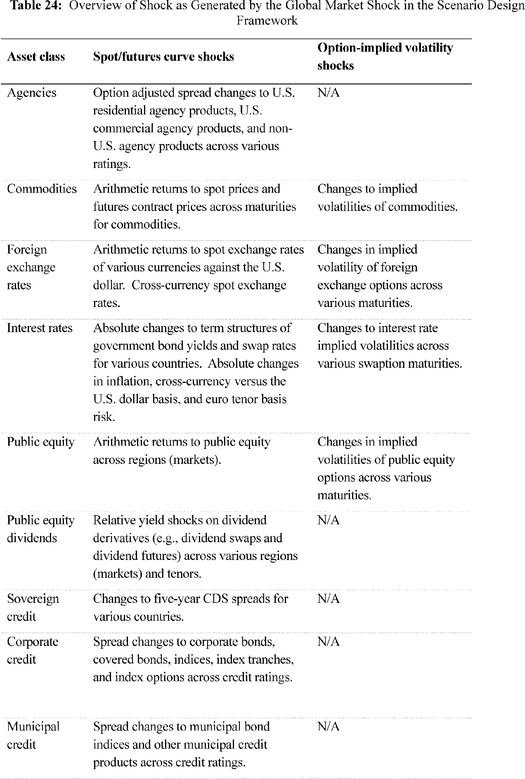

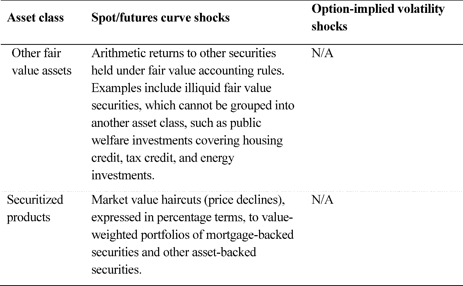
Liquidity Horizons

Financial risk factor shocks are calibrated based on assumed time horizons that reflect several scenario design considerations. The horizons are generally longer than the typical times needed to liquidate exposures under normal conditions because they are designed to capture the unpredictable liquidity conditions that prevail in times of stress. The Board is proposing to add descriptions of the liquidity horizons in the Scenario Design Policy Statement.

As discussed below, the Board is proposing horizons that are intended to maintain consistency with the timeline for attributing losses stemming from these risk factors. Specifically, losses associated with the global market shock component are recognized in the first quarter of the projection horizon, which indicates that these shocks occur within a three-month period and thus implies a three-month upper bound for calibrating the shocks.

The Board is proposing to amend its Scenario Design Policy Statement to use shock liquidity horizons that are broadly consistent with the proposed standards in the Basel Committee on Banking Supervision's Fundamental Review of the Trading Book (FRTB).^[249] The risk factors in the FRTB are similar to the ones in global market shock. The horizons in the FRTB were determined by the Basel Committee in consultations with the financial industry and represent the general consensus of a broad range of regulation authorities and the industry. Therefore, they are a reasonable benchmark for defining the shock horizons used in the global market shock. The Board departed from the FRTB slightly by specifying the same liquidity horizon to all risk factors in the same asset class. This choice was consistent with the Board's stress test principle of simplicity and facilitated a more straightforward modeling framework for the global market shock.

The liquidity horizons used in the global market shock component are not perfectly matched with the FRTB liquidity horizons due to granularity differences between the FRTB standards and the global market shock template. The FRTB specifies horizons at a more granular level, often using different horizons within each asset class. For example, the FRTB specifies sovereign risk factor horizons by credit rating. In contrast, the global market shock template specifies sovereign shocks by country to capture country-specific risks not reflected by credit ratings. Moreover, the Board uses the same liquidity horizon for all risk factors within each asset class, whereas the FRTB allows for different horizons within asset classes. Given these differences, the global market shock scenario aims at aligning with the horizons specified by the FRTB by using a weighted average of the FRTB horizons within each asset class. The weights are determined using aggregate firm exposures over past submission quarters. For example, FRTB horizons for equity risk factors vary between 10 and 60 business days, and the global market shock horizon for this asset class would be four weeks. Because the Board imposes an upper bound on global market shock horizons of one quarter, there are cases where the range of FRTB horizons would be longer than the global market shock horizon. For example, FRTB horizons for corporate credit risk factors vary between 60 and 120 business days, but the Board uses a horizon of three months for corporate credit. See Table 25.

( printed page 51930)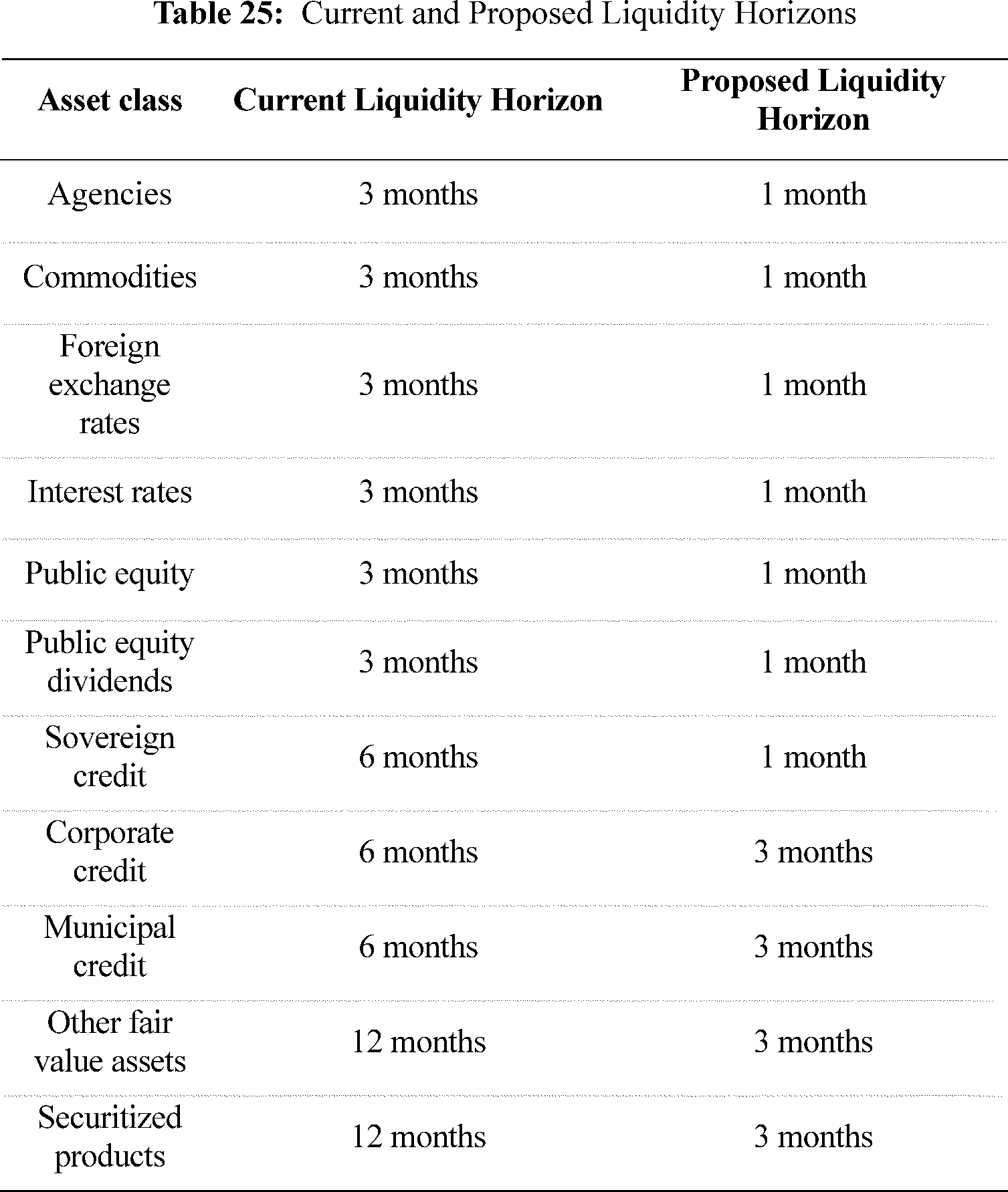

Question 49: What are the advantages and disadvantages of the Board's proposed liquidity horizons? What, if any, additional or alternative liquidity time horizons should the Board consider?

Global Market Shock Simplification

As discussed in Section II.B of this Supplementary Information, the global market shock specifies hypothetical shocks to a standard set of risk factors. Currently, the global market shock discloses more than 20,000 risk factors that reflect sudden market distress and heightened uncertainty. Statistical models are used to generate a subset of risk factors out of these 20,000 risk factors with the remaining ones generated by simple mapping. However, this latter category includes many risk factors that are often not material (for example, certain commodity shocks). These low-materiality exposures do not necessarily enhance the risk capture of the global market shock component.

To address these issues and simplify the global market shock component, the Board is proposing to substantially reduce the number of disclosed risk factors. Specifically, this would reduce the number of disclosed risk factors to approximately 2,300 shocks, determined based on their relevance for developing a global market shock scenario narrative, the materiality of the risk factor, data quality, and consistency across asset classes.

Under this approach, the Board would also review consistency across asset classes. In this regard, where possible, the Board would generate shocks to the same set of countries, regions, and tenor points across different asset classes. Such consistency would simplify shock comparison across different asset classes and improve public understanding of the global market shock component. Additionally, the Board is proposing to remove the inclusion of shocks to the values of private equity positions in section 3.2(b)(viii) of the Scenario Design Policy Statement, because private equity exposures are now stressed using the severely adverse macroeconomic scenario.

Question 50: What are the advantages and disadvantages of simplifying the global market shock's specification of risk factor shocks? What are the advantages and disadvantages of removing shocks related to the value of private equity positions from the global market shock component?

X. Economic Analysis

Introduction

In December 2024, the Board announced that it would seek public ( printed page 51931) comment on significant changes to improve the transparency of its supervisory stress test and to reduce the volatility of resulting capital buffer requirements.^[250] As discussed in Section II.E of this Supplementary Information, this proposal would improve the transparency and public accountability surrounding the stress test models and scenarios, as well as make certain changes to their underlying methodologies, which could provide meaningful benefits to the public as discussed below. This section provides economic analysis of the enhanced disclosure of the supervisory stress test framework.

The Board's supervisory stress test has historically operated with some disclosure regarding the stress test models and scenarios used, with an increase in public information provided beginning in 2019, as discussed in Section II.B of this Supplementary Information. The comprehensive model documentation that the Board is publishing on its website, as well as the proposed enhanced disclosure process for the models and scenarios, provides several benefits, including improved credibility of the stress test, improvement in feedback regarding the modeling process, better informed investors, and improved market discipline. However, the enhanced disclosure comes with costs as well, including reduced model dynamism, and increased systemic reliance on a single model, that is, “model monoculture.”

Baseline

The economic analysis uses the current stress testing framework, including the current disclosure regime, as the baseline. Throughout the analysis, the Board assesses the economic impact of the proposal by comparing outcomes under the proposal to the outcomes estimated under the baseline.

Proposed Policy Changes

With this proposal, the Board is providing a comprehensive description of the modeling framework used to conduct the supervisory stress test: the equations, variables and parameters of each model used to estimate the projections that, when aggregated, produce the results of the supervisory stress test. This proposal would also codify an enhanced disclosure process under which the Board would annually publish the stress test models, invite public comment on any material changes to the models, and seek comment on the annual stress test scenarios. This represents a significant increase in disclosure relative to present, as current stress test disclosures are more limited, for example, current disclosures cover the structure of the stress testing model framework and key variables, along with hypothetical portfolio loss rates for select corporate and retail loss models.

In addition, this proposal would change the stress test jump-off date and the GMS as-of date, as described in Sections VI.A and VI.B of this Supplementary Information. These changes would adjust the stress testing schedule to accommodate the public comment process and mitigate risks that the enhanced disclosure provided under this proposal would undermine the goals of supervisory stress testing.

Section VIII.A of this Supplementary Information summarizes proposed changes to the stress testing models from the 2025 to the 2026 supervisory stress test, which would inform the Board's determination of firms' stress capital buffer requirements.^[251] Section VIII.B provides an analysis of the potential effects of these proposed model changes.

Finally, Sections V and IX of this Supplementary Information describe proposed changes to the Board's Stress Testing Policy Statement and Scenario Design Policy Statement. The proposed changes to the Board's Stress Testing Policy Statement and Scenario Design Policy Statement are intended to express the Board's expectations for how the Board conducts the annual supervisory stress test and designs annual scenarios for the annual supervisory stress test. These changes provide additional transparency, public accountability, and predictability without creating binding legal obligations or economic impact.

Analysis of Benefits and Costs of Enhanced Model Disclosure

Benefits

a. Improved Credibility of the Stress Test

The supervisory stress test has material safety and soundness benefits and these benefits are likely more sustainable when the Board's stress testing program operates with high levels of accountability and credibility. Disclosing comprehensive model documentation to the public ensures that all institutions and stakeholders have equal access to the supervisory methodology, which could improve accountability in supervisory decision-making, promote fairness, and reinforce trust in the stress testing process. Publicly disclosing the stress test models and scenarios also enhances trust in the stress testing process,^[252] as stakeholders may be able to better assess the soundness of models and their alignment with best practices.^[253] As a result, firms may understand better where there are discrepancies between their own internal stress testing models and the supervisory stress testing models, and consequently they may be better positioned to communicate specific concerns with supervisors. With greater transparency and public accountability, stakeholders may be more confident that the supervisory stress test results do not reflect the desires of firms or supervisors to obtain a specific outcome.^[254] While the Board has previously released enhanced disclosures of the stress test models, such as portfolio-level average loss rates, macro-to-loss linkages, and risk drivers, the comprehensive model documentation disclosed in connection with this proposal better illustrates how supervisors incorporate model refinements and emerging risks, which could further improve credibility over time.

In addition, as described in Section VI.B of this Supplementary Information, this proposal would extend the date selection range of GMS as-of date from five months (between October 1 of the previous year and March 1 of a given year) to a full year (between October 1 of two years prior to a given stress test cycle to October 1 of the year prior to a given stress test cycle). Thus, the GMS ( printed page 51932) could be applied to market risk positions held by the firms on any selected date within the full year instead of the current five months. This change could reduce firm's risk gaming activities such as “window dressing” for firms subject to the GMS. Therefore, the resulting improved risk capture would further enhance the credibility of the stress test results.

b. Improved Model Feedback

The Board's supervisory stress test models consist of equations, parameters, and assumptions that translate hypothetical macroeconomic shocks under designed stress scenarios into loss estimates across asset classes, income streams, and capital ratios. Despite their complexity, the supervisory stress test models and stress scenarios, like all theoretical models, remain simplified representations of reality. As such, they benefit from feedback and refinement. Public disclosure of models and scenarios should provide academics, industry professionals, and the broader risk community with the information to provide more effective feedback.^[255] For example, in past supervisory stress testing cycles, stakeholders have raised concerns about loss rates on certain asset classes. Over time, such feedback could help to refine and improve the models and scenarios as they could be updated to mitigate concerns, as appropriate. In this sense, the proposal's enhanced disclosure could facilitate stakeholders' feedback, ultimately leading to better modelling performance and further enhancing the credibility of the supervisory stress testing process.^[256]

c. Improved Ability To Evaluate Business Plans

Comprehensive disclosure of the stress test models also may help firms better understand how supervisors assess losses under severely stressed hypothetical scenarios. This may allow firms to more accurately predict their required capital ratios, reducing capital planning uncertainty ^[257] and possibly increasing firms' willingness to lend.^[258] Reduced capital requirement uncertainty could help firms better plan their future business decisions.

d. Better Informed Investors and Improved Market Discipline

Research suggests that investors use stress test results to assess firms' resilience. Indeed, disclosures of results from the stress test tend to affect firms' stock prices and CDS spreads.^[259] Through such financial market signals, investors may help discipline firms' risk taking.^[260] This “market discipline” may constrain risk taking and incentivize firms to strengthen capital positions.^[261] The comprehensive disclosure of the supervisory stress testing models may allow investors to make better informed decisions, potentially improving the effectiveness of market discipline.

Costs

a. Reduced Dynamism

As discussed above, models are necessarily a simplified version of reality. As forecasting methodologies evolve or conditions in the economy and the financial system change, the existing models may no longer adequately capture risks. For this reason, an effective stress test must be able to adapt. Under this proposal, material changes to the stress testing models would be published for comment, and the Board would be required to respond to such comment, before implementing the material model changes in the supervisory stress test. This process would increase the resources needed to develop, propose, and implement material model changes, particularly to the extent that any changes are complex, present many alternatives, or affect firms' ability to distribute capital. As a result, the use of new models or model changes that explore risks that are less established may pose a high resource burden under the proposed enhanced disclosure regime, potentially limiting the supervisory stress test to simpler, less controversial, and more familiar approaches.^[262] Tests of new risk dimensions or emerging threats may take significantly more time to implement. With less dynamism, the supervisory stress test may fail to capture new risks and could produce an increasingly stale view of how firms would be likely to perform under stressed conditions.^[263] In addition, as described in Section VI.A of this Supplementary Information, this proposal would change the jump-off date of the supervisory and company-run stress tests from December 31 to September 30, to allow the Board to publish the annually disclosed stress test information for comment after the jump-off date of the stress test and to prevent firms from adjusting their exposures based on the published information. As a result, the tested balance sheets would be older by one quarter, which would add additional staleness to the stress test and stress test results, because firm balance sheets as well as economic conditions could change substantially within a quarter.

b. Reduced Risk Sensitivity and Overreliance on a Single Model Framework

Supervisory stress testing results are important inputs to the capital requirements associated with firms' ( printed page 51933) banking activities. With comprehensive model disclosure likely reducing the uncertainty of supervisory stress test results, firms' estimates of future regulatory capital requirements could rely more on the Board's stress test models and less on their own internal stress testing models or internal risk management tools, both of which may be less useful than before for managing regulatory capital.^[264] To the extent that firms' own internal stress testing models or risk management tools provide additional information about risk, the expected capital requirements could become less risk-sensitive as a result and it may reduce firms' incentives to independently measure and manage their vulnerabilities.

Disclosure could also enable firms to more easily optimize their exposures to minimize capital requirements in the supervisory stress test, which could allow vulnerabilities to build up where risks are not well or fully accounted for by standardized supervisory models.

Reliance on the supervisory stress testing models could extend further if disclosure results in firms increasing the similarity of their own stress models to the stress test models.^[265] Increased reliance of all stress tested firms on a single model, known as “model monoculture,” or delaying material model changes while risks build up in areas that are treated benignly in the stress test would pose risks, as firms may face a greater incentive to shift business activities towards these areas to reduce their capital requirements.^[266] The resulting convergence of risk taking could increase the vulnerability of the banking system, particularly to those risks that are under-reflected by the supervisory stress testing models.^[267]

Conclusion

As discussed in the introduction to Section X.D of this Supplementary Information, the Board's supervisory stress test has historically operated with partial disclosure regarding the stress test models used. The comprehensive model documentation published in connection with this proposal, as well as the proposed enhanced disclosure process, provides several benefits that outweigh the costs of the proposal.

Taken together, the Board assessed that the benefits of the proposal justify the costs.

Question 51: What, if any, additional material costs or benefits should the Board consider, in addition to those discussed in the proposal?

Question 52: What alternatives that achieve the objectives of the proposal should the Board evaluate? Please provide specific suggestions and rationales for any proposed alternatives, including how they might address potential unintended consequences or better achieve the proposal's goals.

XI. Administrative Law Matters

A. Paperwork Reduction Act Analysis

In accordance with the requirements of the Paperwork Reduction Act (PRA) of 1995 (44 U.S.C. 3501-3521), the Board may not conduct or sponsor, and the respondent is not required to respond to, an information collection unless it displays a currently valid Office of Management and Budget (OMB) control number. The Board reviewed the information collections related to the proposed rule under the authority delegated to the Board by OMB.

The proposed rule would not create any information collections subject to the PRA; however, the Board is proposing to revise the FR Y-14A/Q/M to reduce regulatory reporting burden by retiring items and removing supporting documentation requirements that are no longer needed to conduct the supervisory stress test. Additionally, the Board is proposing to collect additional information to support the proposed supervisory stress test models.

The Board invites public comment on the following information collection:

(a) Whether the collection of information is necessary for the proper performance of the Board's functions, including whether the information has practical utility;

(b) The accuracy of the Board's estimate of the burden of the proposed information collection, including the validity of the methodology and assumptions used;

(c) Ways to enhance the quality, utility, and clarity of the information to be collected;

(d) Ways to minimize the burden of the information collection on respondents, including through the use of automated collection techniques or other forms of information technology; and

(e) Estimates of capital or start-up costs and costs of operation, maintenance, and purchase of services to provide information.

Proposal Under OMB Delegated Authority To Extend for Three Years, With Revision, the Following Information Collection

Collection title: Capital Assessments and Stress Testing Reports.

Collection identifier: FR Y-14A/Q/M.

OMB control number: 7100-0341.

General description of collection: This family of information collections is composed of the following three reports:

• The annual FR Y-14A collects quantitative projections of balance sheet, income, losses, and capital across a range of macroeconomic scenarios and qualitative information on methodologies used to develop internal projections of capital across scenarios.^[268]

• The quarterly FR Y-14Q collects granular data on various asset classes, including loans, securities, trading assets, and pre-provision net revenue for the reporting period.
• The monthly FR Y-14M is comprised of three retail portfolio- and loan-level schedules, and one detailed address-matching schedule to supplement two of the portfolio- and loan-level schedules. ( printed page 51934)

The data collected through the FR Y-14A/Q/M provide the Board with the information needed to help ensure that large firms have strong, firm-wide risk measurement and management processes supporting their internal assessments of capital adequacy and that their capital resources are sufficient, given their business focus, activities, and resulting risk exposures. The data within the reports are used in connection with setting firms' stress capital buffer requirements. The data are also used to support other Board supervisory efforts aimed at enhancing the continued viability of large firms, including continuous monitoring of firms' planning and management of liquidity and funding resources, as well as regular assessments of credit risk, market risk, and operational risk, and associated risk management practices. Information gathered in this collection is also used in the supervision and regulation of respondent financial institutions. Respondent firms are currently required to complete and submit up to 17 filings each year: one annual FR Y-14A filing, four quarterly FR Y-14Q filings, and 12 monthly FR Y-14M filings.^[269] Compliance with the information collection is mandatory.

Current Actions: The proposal would modify the FR Y-14A/Q/M to remove supporting documentation requirements, schedules, and data items that are no longer needed to conduct the supervisory stress test. The proposal would also make other revisions necessary to facilitate the stress test modeling decisions. All proposed revisions would be effective for the September 30, 2026, report date.

Supporting Documentation

a. FR Y-14A

The FR Y-14A collects detailed data on firms' quantitative projections of assets, liabilities, income, losses, and capital across a range of macroeconomic scenarios. Firms are also required to provide qualitative information on the methodologies used to develop their projections and any other analysis that supports or contributes to these projections. This qualitative supporting documentation helps supervisors assess the accuracy and comprehensiveness of the projections included in firms' FR Y-14A submissions. This information was previously critical to assess the data systems and modeling methodologies that firms used to report the FR Y-14A. However, as these systems and frameworks have matured, much of the supporting documentation has become outdated or is not needed by supervisors to make such assessments. To ensure that the FR Y-14A requirements do not capture information that is no longer needed and to reduce reporting burden, the Board is proposing to remove Appendix A “Supporting Documentation” from the FR Y-14A. However, supervisors may request similar information to what is currently required from Appendix A from firms through supervisory channels, as deemed appropriate and on a targeted basis, in support of the annual capital plan review. Firms would only be expected to provide information that supervisors request each cycle. The proposed removal of the FR Y-14A supporting documentation reporting requirement would not impact any other capital planning expectations.

b. FR Y-14Q

FR Y-14Q, Schedule L (Counterparty) collects data on firms' counterparty credit risk, including derivative and securities financing transaction exposures. Applicable firms are required to report two versions of Schedule L: an “unstressed” version under the actual economic conditions on the reported date, and a “stressed” version under the hypothetical stress scenarios used in the supervisory and company-run stress tests. To support firms' estimates of credit valuation adjustment and counterparty losses under the stress scenarios, the FR Y-14Q requires that firms provide detailed descriptions of the methodologies used to generate values for the “stressed” version. As for the FR Y-14A, this information was previously important in understanding firms' counterparty submissions but is no longer required for supervisors to assess Schedule L data. However, the Board has identified supporting information that is relevant to understanding a firm's estimated credit valuation adjustment and largest counterparty default losses. Therefore, to streamline Schedule L and reduce reporting burden, the Board is proposing replacing the existing Schedule L supporting documentation with this more limited set of questions. These questions would concern excluded counterparties, estimation assumptions, drivers of changes in credit valuation adjustment, and other related topics.

Similarly, qualitative information is needed to assess firms' trading mark-to-market projections under the global market shock. As a firm's projections are directly connected to the exposures reported on FR Y-14Q, Schedule F (Trading), the Board is proposing to introduce supporting documentation for Schedule F that includes five questions related to a firm's trading projections and Schedule F submissions. Together with the Schedule L supporting documentation, this would ensure that supervisors have the necessary information to assess a firm's projections under the global market shock.

Home Equity Data Collection

FR Y-14M, Schedule B.1 (Home Equity Loan-Level Table) collects loan-level data on firms' HELOCs. These data are used in support of stress test modeling and monitoring of firms' home equity portfolios. The Board has identified several items on Schedule B.1 that are not needed to assess a home equity loan or HELOC's risk characteristics or are captured elsewhere on Schedule B.1. Therefore, to maintain appropriate risk coverage and reduce reporting burden, the Board is proposing to retire the following fields from Schedule B.1.

• Item 18 (Number of Units)
• Item 31 (ARM Periodic Rate Cap)
• Item 32 (ARM Periodic Rate Floor)
• Item 38 (Bankruptcy Flag)
• Item 48 (Foreclosure Referral Date)
• Item 51 (Pre-Payment Penalty Term)
• Item 58 (Interest Rate Frozen)
• Item 59 (Principal Deferred)
• Item 62 (First Mortgage Serviced in House)
• Item 72 (Term Modification)
• Item 73 (Principal Write-Down)
• Item 74 (Line Re-Age)
• Item 75 (Loan Extension)
• Item 86 (Accrual Status)
• Item 87 (Foreclosure Suspended)
• Item 88 (Property Valuation Method at Origination)
• Item 92 (Third Party Sale Flag)
• Item 107 (Entity Type)

Collection of Mailing Address Information

FR Y-14M, Schedule C (Address Matching) collects address information on each loan reported on FR Y-14M, Schedule A (First Lien) or Schedule B (Home Equity). This collection includes both property and mailing address data used in support of the supervisory stress test models. However, the Board has determined that the mailing address items are no longer needed for stress testing or supervisory purposes. Therefore, the Board is proposing to remove item 6 (Mailing Stress Address), item 7 (Mailing City), item 8 (Mailing State), and item 9 (Mailing Zip Code) from Schedule C. ( printed page 51935)

Unpaid Principal Balance

FR Y-14M, Schedule B.1 item 95 (Unpaid Principal Balance (Net)) collects information on the current net unpaid principal balance of a home equity line of credit. The instructions provide a definition for calculating net unpaid principal balance and note that this value should equal the book value on regulatory filings. However, reporting of unpaid principal balance can vary across regulatory reporting, including by considering loan premiums, which item 95 does not include. To address this inconsistency, the Board is proposing to remove this language from the instructions for item 95.

Private Equity

Beginning with the 2025 supervisory stress test, the Board calculated losses on private equity exposures under the macroeconomic scenario over a nine-quarter projection horizon as opposed to under the GMS, which would have considered the impact only in the first quarter of the projection horizon. As described in the Board's 2025 Supervisory Stress Test Methodology disclosure,^[270] the new treatment better aligns with the characteristics of private equity exposures, which are principally long-term investments that are managed as banking book positions. To better capture private equity data in a manner that aligns with this new treatment, the Board is proposing several revisions to FR Y-14Q, Schedule F (Trading).

First, the Board is proposing to move the fourth quarter as-of date for reported private equity exposures to December 31 of a given year, as opposed to the as-of date of the GMS. Schedule F is reported on a quarterly basis. However, to gather data necessary to subject firms to the GMS, firms are required to report Schedule F as of the GMS as-of date and not as of December 31 for the fourth quarter submission. Therefore, the Board is proposing to require private equity exposures to be reported as of December 31, as private equity exposures are no longer stressed under the GMS.

Second, the Board is proposing to revise Schedule F such that private equity carry values are reported net of embedded goodwill or investments in the capital of unconsolidated financial institutions that are deducted from common equity tier 1 capital. The Board's capital rule provides that certain amounts of goodwill and investments in the capital of unconsolidated financial institutions be deducted from CET1 capital,^[271] and the carry value of private equity exposures reported on Schedule F can be affected by these deducted amounts.

Firms subject to Category I through III standards are required to report these deduction items on FR Y-14A, Schedule A.1.d (Capital). To ensure that deductions are not double-counted when calculating trading and counterparty losses, firms may report an adjusted starting value for these items to reflect the impact of the global market shock. However, as currently reported, a portion of these amounts may be attributable to private equity. Therefore, the Board is proposing revising Schedule F to require firms to exclude the amounts attributable to private equity from the carry value. This revision would ensure that losses are not assigned to balances that have been deducted from capital when calculating private equity losses.

Third, the Board is proposing to require hedges on private equity exposures to be separately reported on Schedule F. Hedges on private equity exposures are currently reported on Schedule F but are not segmented from other hedges on trading exposures. Given that private equity exposures are no longer stressed as part of the GMS, the Board is proposing to require hedges on private equity exposures to be reported separately so that they can be considered as part of the macroeconomic scenario.

Lastly, the Board is proposing to implement a new materiality threshold for the reporting of Schedule F.24 (Private Equity). Currently, Schedule F.24 is reported only by firms subject to Category I through III standards with substantial trading operations, which is defined as having, on average for four quarters, aggregate trading assets and liabilities of $50 billion or more, or aggregate trading assets and liabilities equal to 10 percent or more of total consolidated assets. However, private equity exposures are primarily banking book positions for which the FR Y-14 uses a separate reporting threshold. For firms subject to Category IV standards, material portfolios for banking book positions are defined as those with asset balances greater than $5 billion or with asset balances greater than ten percent of tier 1 capital on average for the four quarters preceding the reporting period. For firms subject to Category I through III standards, material portfolios for banking book positions are defined as those with asset balances greater than $5 billion or asset balances greater than five percent of tier 1 capital on average for the four quarters preceding the reporting period.

To align the materiality threshold for private equity with other banking book schedules, the Board is proposing to revise the FR Y-14Q instructions to apply the materiality threshold to Schedule F.24 that is currently applied to the banking book schedules. Additionally, since a firm subject to Category IV standards could have its private equity losses contribute to its supervisory stress test results, the Board also proposes to require a firm subject to Category IV standards to submit Schedule F.24 if it meets the proposed materiality threshold. Similarly, consistent with reporting expectations for other banking book positions, the Board is proposing to update FR Y-14Q, Schedule K (Supplemental) such that firms report the carrying value of funded and unfunded private equity exposures that do not meet the materiality threshold for Schedule F.24 reporting. These revisions would ensure consistent reporting and treatment of private equity in the supervisory stress test.

Additionally, the Board is proposing a revision to FR Y-14A, Schedule A.4 (Trading) which captures trading profit and loss projections under the global market shock. As private equity shocks are no longer included in the global market shock, items related to private equity are no longer needed to capture trading profit and loss projections. Therefore, the Board is proposing to remove item 15 (“Private Equity”), item 15A (“Private Equity: Funded”), item 15B (“Private Equity: Unfunded”), item 15C (“Private Equity: Other”) from Schedule A.4.

Other Hedges

Currently, the FR Y-14Q captures certain types of hedges, including hedges on accrual loans and loans held under the fair value option and certain designated accounting hedges on securities, but is not comprehensive, which limits the ability of the supervisory stress test to account for these positions. For example, FR Y-14Q, Schedule B (Securities) does not provide sufficient information to independently revalue the hedging instrument. Additionally, interest rate risk hedges that are used to mitigate risk on instruments other than securities from changes in interest rates are not captured by the FR Y-14Q. Schedule B was designed to capture basic information on traditional hedges on securities and does not consistently and comprehensively capture portfolio layer ( printed page 51936) method or interest rate risk hedges for valuation purposes.

Separately, fair value option hedges are positions that are used to hedge loan assets that are held-for-sale or held under fair value option accounting, and do not meet the definition of trading assets or liabilities. This includes synthetic securitizations, a form of loss mitigation in which a firm partially transfers credit risk on specific portfolios to outside investors through credit derivatives or guarantees. Fair value option hedges are currently reported as a separate instance of Schedule F. However, Schedule F is subject to a materiality threshold, so fair value option hedges are not reported comprehensively by all relevant firms on the FR Y-14Q.

To improve the risk capture of the supervisory stress test by incorporating the effects of additional hedges, the Board is proposing to revise FR Y-14Q, Schedule B.2 (Investment Securities with Designated Accounting Hedges) to capture all qualified accounting hedges, including portfolio layer method and all designated accounting hedges. Additionally, the Board is proposing to implement FR Y-14Q, Schedule B.3 to more comprehensively map hedging relationships. Similarly, the Board is proposing to revise Schedule F to capture data on hedges from any firms with reportable hedges.

Question 53: Would the new fields proposed in FR Y-14Q, Schedule B.2 or B.3 prove burdensome to report for firms?

Question 54: Do the new fields proposed in FR Y-14Q, Schedule B.2 provide sufficient information to independently model the value of the hedging instrument?

Question 55: Should changes be made to the fields or definitions proposed in FR Y-14Q, Schedule B.2 to better account for more esoteric derivatives such as swaptions, cap, or floors?

Exchange Traded Funds

Exchange traded funds (ETFs) are investment funds comprised of exposures to multiple underlying assets, such as commodities, equities, or currencies. Currently, Schedule F instructs firms to decompose certain ETF exposures based on the fund's underlying assets. However, the instructions also provide that all other ETFs should be reported in the equity worksheets. This ambiguity may lead to classifying non-equity ETFs in the equity worksheets.

All ETFs should be reported based on the underlying asset holdings and associated risk factors. For example, ETFs for which rates or credit exposures are the underlying holdings should be reported on the corresponding worksheet. To provide clarity and ensure consistent reporting, the Board is proposing to clarify the Schedule F instructions such that all ETFs are reported in the worksheet that corresponds to the underlying asset class and risk exposures.

Credit Card Revenue and Loss Share Agreements

Revenue and loss sharing agreements (RLSAs) are partnership agreements firms have with private entities to share a portion of profits, revenues, and/or losses generated by a specified asset. As discussed in the Credit Cards Model description, the Board accounts for private RLSAs when projecting credit card losses in the supervisory stress test. Currently, the Board's adjustment accounts for a specific case where a firm accounts for loss sharing payments by reducing provisions. However, as agreement terms and reporting practices vary, the current adjustment may not fully or consistently address differential RLSA treatment across firms. Therefore, the Board is considering additional enhancements to the current RLSA adjustment to more comprehensively capture RLSAs in the supervisory stress test. Specifically, the Board is considering one modeling approach that would account for RLSAs at the portfolio level and a second that would account for RLSAs at the agreement level. To facilitate the portfolio level enhancement, the Board is proposing to collect portfolio level details on FR Y-14M, Schedule D (Credit Card) of individual revenue components ( e.g., interest income, interest expense, noninterest income, and noninterest expense), charge-offs and recoveries, and provision build. Additionally, the amount of each that is subject to partner sharing agreements and where the partner shares portions of each are reported on the FR Y-9C, as well as the shared amounts of net profit, net revenue, and net charge offs. To facilitate the agreement level enhancement, the Board is proposing to collect the same information at the agreement level, as well as effective share rates and contractual share rates of the individual revenue, loss, and provision components. For both approaches, the Board is proposing to expand Schedule D.1, item 70 (“Loss Sharing”) to collect information on the type of RLSA. If either the portfolio level or agreement level enhancement is adopted, the Board would only adopt the corresponding FR Y-14 revisions. If the Board does not adopt either enhancement to the RLSA adjustment, then neither set of revisions would be implemented. If either RLSA modeling enhancement is adopted, the corresponding FR Y-14 revision would represent an increase in estimated FR Y-14 burden hours of approximately 2,500 hours if adopted.

Stress Test Date Changes

a. FR Y-14A Jump-Off Date

The FR Y-14A collects data on firms' projections of balance sheet asset and liabilities, income, losses, and capital across a range of hypothetical scenarios. These projections span a nine-quarter horizon beginning with the first quarter of the year in which the report is filed. This means that the jump-off date for the FR Y-14A is December 31 of the previous year, consistent with the supervisory stress test. However, as discussed in Section VI.A of this Supplementary Information, the Board is proposing to shift the jump-off date of the stress test to September 30 so that the scenarios are released for comment after the finalization of firms' balance sheets.

Consistent with this proposed jump-off date change, the Board is proposing to modify the FR Y-14A to use a September 30 jump-off date. These revisions would include updating the instructions to note that the projection horizon begins in the fourth quarter of the year preceding the reporting year, and noting that firms should report actual capital actions in the first and second quarters of the projection horizon, as they occur before the due date. The FR Y-14A and capital plans would still be due April 5.

b. Global Market Shock as-of Date Submissions

As discussed in Section VI.B of this Supplementary Information, the Board is proposing to expand the as-of date range for the global market shock to be between October 1 of two years prior to a given stress test cycle to October 1 of the year prior to a given stress test cycle. To facilitate this proposed change, the Board is proposing several changes to the FR Y-14A and FR Y-14Q.

On the FR Y-14A, the Board is proposing to update Schedule A.4 (Trading) and Schedule A.5 (Counterparty) such that the as-of date for these schedules may fall between October 1 of two years prior to a given stress test cycle to October 1 of the year prior to a given stress test cycle. These schedules would still be due on April 5 of the following year.

( printed page 51937)

Currently, the fourth quarter submissions of FR Y-14Q, Schedule F (Trading) and Schedule L (Counterparty) are submitted as of the global market shock as-of date instead of quarter end. However, under the proposal, the as-of date for the global market shock could fall in a quarter other than the fourth quarter. Therefore, Board is proposing to modify the submission cadence for Schedule F (Trading) and Schedule L (Counterparty) such that, for whichever quarter contains the global market shock as-of date, Schedule F and Schedule L would be submitted as of that date, as opposed to quarter end. Submissions for all other quarters would be submitted as-of quarter end.

Question 56: What, if any, other FR Y-14 revisions are needed to facilitate the proposed changes to the stress test jump-off date and global market shock as-of date?

Frequency: Annually, quarterly, and monthly.

Respondents: Holding companies with $100 billion or more in total consolidated assets, as based on (1) the average of the firm's total consolidated assets in the four most recent quarters as reported quarterly on the firm's Consolidated Financial Statements for Holding Companies (FR Y-9C; OMB No. 7100-0128) or (2) the average of the firm's total consolidated assets in the most recent consecutive quarters as reported quarterly on the firm's FR Y-9Cs, if the firm has not filed an FR Y-9C for each of the most recent four quarters.

Total estimated number of respondents: 35.

Estimated change in burden:

• FR Y-14A: −4,235 hours.
• FR Y-14Q: −700 hours.
• FR Y-14M: +792 hours.
• Total estimated change in burden: −4,143.

Total estimated annual burden hours: 757,696.

B. Regulatory Flexibility Act Analysis

The Board is providing an initial regulatory flexibility analysis with respect to this proposed rule. The Regulatory Flexibility Act (RFA) ^[272] requires an agency to consider whether the rules it proposes will have a significant economic impact on a substantial number of small entities.^[273] In connection with a proposed rule, the RFA requires an agency to prepare and invite public comment on an initial regulatory flexibility analysis describing the impact of the rule on small entities, unless the agency certifies that the proposed rule, if promulgated, will not have a significant economic impact on a substantial number of small entities. An initial regulatory flexibility analysis must contain (1) a description of the reasons why action by the agency is being considered; (2) a succinct statement of the objectives of, and legal basis for, the proposed rule; (3) a description of, and, where feasible, an estimate of the number of small entities to which the proposed rule will apply; (4) a description of the projected reporting, recordkeeping, and other compliance requirements of the proposed rule, including an estimate of the classes of small entities that will be subject to the requirement and the type of professional skills necessary for preparation of the report or record; (5) an identification, to the extent practicable, of all relevant Federal rules which may duplicate, overlap with, or conflict with the proposed rule; and (6) a description of any significant alternatives to the proposed rule which accomplish the stated objectives of applicable statutes and minimize any significant economic impact of the proposed rule on small entities.

The Board has considered the potential impact of the proposed rule on small entities in accordance with the RFA. Based on its analysis and for the reasons stated below, the Board believes that this proposed rule will not have a significant economic impact on a substantial number of small entities. Nevertheless, the Board is publishing and inviting comment on this initial regulatory flexibility analysis. In connection with this proposal, the Board also proposes to make changes to the Board's reporting forms.

As discussed in detail above, under the proposal, the Board is inviting public comment on the models used to conduct the Board's supervisory stress test, changes to those models to be implemented in the 2026 stress test, and proposed changes to enhance the transparency and public accountability of the Board's stress testing framework. The proposal would amend the Policy Statement on the Scenario Design Framework for Stress Testing, including to implement guides for additional scenario variables, and the Stress Testing Policy Statement. The proposal would also codify an enhanced disclosure process under which the Board would annually publish comprehensive documentation on the stress test models, invite public comment on any material changes that the Board seeks to make to those models, and annually publish the stress test scenarios for comment. Lastly, the proposal would make changes to the FR Y-14A/Q/M to remove items that are no longer needed to conduct the supervisory stress test and to collect additional data to support the stress test models and improve risk capture.

As discussed above, several statutory authorities, including the International Lending Supervision Act of 1983,^[274] section 5(b) of the Bank Holding Company Act,^[275] the International Banking Act,^[276] section 10(g) of the Home Owners' Loan Act,^[277] and section 165 of the Dodd-Frank Wall Street Reform and Consumer Protection Act (Dodd-Frank Act) ^[278] (as amended by section 401 of the Economic Growth, Regulatory Relief, and Consumer Protection Act ^[279] ), provide authority for the Board's stress testing and stress capital buffer framework, including this proposed rule.

The International Lending Supervision Act of 1983 provides the Board with broad discretionary authority to set minimum capital levels for state member banks and affiliates of insured depository institutions, including holding companies, supervised by the Board.^[280] Under section 5(b) of the Bank Holding Company Act, the Board may issue such regulations and orders relating to capital requirements of bank holding companies as may be necessary for the Board to carry out the purposes of the Bank Holding Company Act.^[281] Foreign banking organizations with a U.S. subsidiary bank, branch, or agency are made subject by the International Banking Act to the provisions of the Bank Holding Company Act in the same manner as bank holding companies; ^[282] therefore, the Board is also authorized under section 5(b) of the Bank Holding Company Act to impose these ( printed page 51938) requirements on those foreign banking organizations.

Similarly, with regard to savings and loan holding companies, section 10(g) of the Home Owners' Loan Act authorizes the Board to issue such regulations and orders relating to capital requirements as the Board deems necessary and appropriate to carry out the purposes of the Home Owners' Loan Act.^[283] Moreover, section 165 of the Dodd-Frank Act, as amended by section 401 of the Economic Growth, Regulatory Relief, and Consumer Protection Act, requires the Board to establish risk-based capital requirements for large bank holding companies and nonbank financial companies supervised by the Board.^[284] Additionally, section 165(i)(1) of the Dodd-Frank Act, as amended by section 401 of the Economic Growth, Regulatory Relief, and Consumer Protection Act, requires the Board to conduct an annual supervisory stress test of these large firms.^[285]

The proposed rule would apply to bank holding companies, U.S. intermediate holding companies of foreign banking organizations, and savings and loan holding companies, each with at least $100 billion in total consolidated assets, as well as state member banks with more than $250 billion in total consolidated assets, certain nonbank financial companies supervised by the Board, and any other bank holding company or covered savings and loan holding company domiciled in the United States that is made subject to the capital plan rule by order of the Board.^[286] The proposed rule would not apply to any small entities. Further, although the Board does not project there to be a direct impact to reporting, recordkeeping, or other compliance requirements as a result of the proposed rule, the Board also is proposing to revise the FR Y-14A/Q/M (Capital Assessments and Stress Testing) reports to remove items that are no longer needed to conduct the supervisory stress test and to collect data that would improve the calculation of the stress capital buffer requirement. These reports are submitted by firms subject to the Board's capital plan rule requirements; thus, the changes would not impact small entities. In addition, the Board is aware of no other Federal rules that duplicate, overlap, or conflict with the proposed changes to the capital and stress testing rules. Accordingly, the Board believes that the proposed rule will not have a significant economic impact on a substantial number of small banking organizations supervised by the Board and, therefore, believes that there are no significant alternatives to the proposed rule that would reduce the economic impact on small banking organizations supervised by the Board.

The Board welcomes comment on all aspects of its analysis.

C. Plain Language

Section 722 of the Gramm-Leach-Bliley Act (Pub. L. 106-102, 113 Stat. 1338, 1471, 12 U.S.C. 4809) requires the federal banking agencies to use plain language in all proposed and final rules published after January 1, 2000. The Board has sought to present the notice of proposed rulemaking in a simple and straightforward manner and invites comment on the use of plain language. For example:

• Is the material organized to suit your needs? If not, how could the Board present the proposed rule more clearly?
• Are the requirements in the proposed rule clearly stated? If not, how could the proposed rule be more clearly stated?
• Does the proposal contain technical language or jargon that is not clear? If so, which language requires clarification?
• Would a different format (grouping and order of sections, use of headings, paragraphing) make the proposed rule easier to understand? If so, what changes would achieve that?
• Is this section format adequate? If not, which of the sections should be changed and how?
• What other changes can the Board incorporate to make the proposed rule easier to understand?

D. Providing Accountability Through Transparency Act of 2023

The Providing Accountability Through Transparency Act of 2023 (12 U.S.C. 553(b)(4)) requires that a notice of proposed rulemaking include the internet address of a summary of not more than 100 words in length of the proposed rule, in plain language, that shall be posted on the internet website under section 206(d) of the E-Government Act of 2002 (44 U.S.C. 3501 note).

The proposal and such a summary can be found at https://www.regulations.gov and https://www.federalreserve.gov/​supervisionreg/​reglisting.htm.

Authority and Issuance

For the reasons stated in the preamble, the Board of Governors of the Federal Reserve System proposes to amend 12 CFR chapter II as follows:

1. The authority citation for part 225 continues to read as follows:

Authority: 12 U.S.C. 1817(j)(13), 1818, 1828(o), 1831i, 1831p-1, 1843(c)(8), 1844(b), 1972(1), 3106, 3108, 3310, 3331-3351, 3906, 3907, and 3909; 15 U.S.C. 1681s, 1681w, 6801 and 6805.

2. In § 225.8:

a. Revise paragraph (d)(16).

b. Remove the text “final,” and add in its place the text “third,” in subparagraph (f)(2)(i)(A).

c. In paragraphs (f)(2)(i)(C)(1), (f)(4), (h)(2)(ii)(A), (h)(2)(ii)(A)(1), (h)(2)(ii)(A)(2), (h)(2)(ii)(B), (h)(2)(ii)(B)(1), and (h)(2)(ii)(B)(2), remove the text “fourth through seventh”, wherever it appears and add in its place the text “fifth through eighth”.

d. In paragraph (k)(2), remove the text “fourth” and replace with the text “fifth.”

The revisions read as follows:

3. The authority citation for part 238 continues to read as follows:

Authority: 5 U.S.C. 552, 559; 12 U.S.C. 1462, 1462a, 1463, 1464, 1467, 1467a, 1468, 5365; 1813, 1817, 1829e, 1831i, 1972; 15 U.S.C. 78l.

4. In § 238.130:

a. Add definitions of Material model change, Model change, and Models.

b. Revise definition of Planning horizon.

5. In § 238.132:

a. Revise paragraph (b).

b. Add subsection (e).

The revisions read as follows:

7. In § 238.141:

a. Revise the definition of Planning horizon.

8. In § 238.143:

a. Revise subparagraph (b)(2)(i).

b. Revise subparagraph (b)(4)(i).

The revisions read as follows:

9. In § 238.170:

a. Revise paragraph (d)(14).

b. Remove the text “final,” and add in its place the text “third,” in subparagraph (f)(2)(i)(A).

c. In paragraphs (f)(2)(i)(C)(1), (f)(4), (h)(2)(ii)(A), (h)(2)(ii)(A)(1), (h)(2)(ii)(A)(2), (h)(2)(ii)(B), (h)(2)(ii)(B)(1), and (h)(2)(ii)(B)(2), remove the text “fourth through seventh”, wherever it appears and add in its place the text “fifth through eighth”.

d. In paragraph (k)(2), remove the text “fourth” and replace with the text “fifth.”

The revisions read as follows:

(d) * * *

(14) Planning horizon means the period of at least nine consecutive quarters, beginning with the quarter two quarters preceding the quarter in which the covered savings and loan holding company submits its capital plan, over which the relevant projections extend.

(f) * * *

(2) * * *

(i) * * *

(A) The ratio of a covered savings and loan holding company's common equity tier 1 capital to risk-weighted assets, as calculated under 12 CFR part 217, subpart D, as of the third quarter of the previous capital plan cycle, unless otherwise determined by the Board; minus

(C) * * *

(1) The sum of the covered savings and loan holding company's planned common stock dividends (expressed as a dollar amount) for each of the fifth through eighth quarters of the planning horizon; to

(4) Adjustment of stress capital buffer requirement. In each calendar year in which the Board does not calculate a Category IV savings and loan holding company's stress capital buffer requirement pursuant to paragraph (f)(1) of this section, the Board will adjust the Category IV savings and loan holding company's stress capital buffer requirement to be equal to the result of the calculation set forth in paragraph (f)(2) of this section, using the same values that were used to calculate the stress capital buffer requirement most recently provided to the covered savings and loan holding company, except that the value used in paragraph (f)(2)(i)(C)(1) of the calculation will be equal to the covered savings and loan holding company's planned common stock dividends (expressed as a dollar amount) for each of the fifth through eighth quarters of the planning horizon as set forth in the capital plan submitted by the covered savings and loan holding company in the calendar year in which the Board adjusts the covered savings and loan holding company's stress capital buffer requirement.

(h) * * *

(2) * * *

(ii) * * * ( printed page 51941)

(A) Determine whether the planned capital distributions for the fifth through eighth quarters of the planning horizon under the Internal baseline scenario would be consistent with effective capital distribution limitations assuming the stress capital buffer requirement provided by the Board under paragraph (h)(1) or (i)(5) of this section, as applicable, in place of any stress capital buffer requirement in effect; and

(1) If the planned capital distributions for the fifth through eighth quarters of the planning horizon under the Internal baseline scenario would not be consistent with effective capital distribution limitations assuming the stress capital buffer requirement provided by the Board under paragraph (h)(1) or (i)(5) of this section, as applicable, in place of any stress capital buffer requirement in effect, the covered savings and loan holding company must adjust its planned capital distributions such that its planned capital distributions would be consistent with effective capital distribution limitations assuming the stress capital buffer requirement provided by the Board under paragraph (h)(1) or (i)(5) of this section, as applicable, in place of any stress capital buffer requirement in effect; or

(2) If the planned capital distributions for the fifth through eighth quarters of the planning horizon under the Internal baseline scenario would be consistent with effective capital distribution limitations assuming the stress capital buffer requirement provided by the Board under paragraph (h)(1) or (i)(5) of this section, as applicable, in place of any stress capital buffer requirement in effect, the covered savings and loan holding company may adjust its planned capital distributions. A covered savings and loan holding company may not adjust its planned capital distributions to be inconsistent with the effective capital distribution limitations assuming the stress capital buffer requirement provided by the Board under paragraph (h)(1) or (i)(5) of this section, as applicable; and

(B) Notify the Board of any adjustments made to planned capital distributions for the fifth through eighth quarters of the planning horizon under the Internal baseline scenario.

(k) * * *

(2) The dollar amount of the capital distribution will exceed the dollar amount of the covered savings and loan holding company's final planned capital distributions, as measured on an aggregate basis beginning in the fifth quarter of the planning horizon through the quarter at issue.

10. The authority citation for part 252 continues to read as follows:

Authority: 12 U.S.C. 321-338a, 481-486, 1467a, 1818, 1828, 1831n, 1831o, 1831p-1, 1831w, 1835, 1844(b), 1844(c), 3101 et seq., 3101 note, 3904, 3906-3909, 4808, 5361, 5362, 5365, 5366, 5367, 5368, 5371.

11. In § 252.12:

a. Revise the definition of Planning Horizon.

12. In § 252.14:

a. Revise subparagraph (b)(2)(i).

b. Revise subparagraph (b)(4)(i).

The revisions read as follows:

13. In § 252.42:

a. Add definitions of Material model change, Model change, and Models.

b. Revise the definition of Planning Horizon.

14. In § 252.44:

a. Revise paragraph (b).

b. Add subsection (e).

The revisions read as follows:

16. In § 252.52:

a. Revise the definition of Planning horizon.

17. In § 252.54:

a. Revise subparagraph (b)(2)(i).

b. Revise subparagraph (b)(4)(i).

The revisions read as follows:

18. Appendix A to part 252 is revised to read as follows:

1. Background

(a) The Board has imposed stress testing requirements through its regulations (stress test rules) implementing section 165(i) of the Dodd-Frank Wall Street Reform and Consumer Protection Act (Dodd-Frank Act or Act), section 10(g) of the Home Owners' Loan Act, and section 401(e) of the Economic Growth, Regulatory Relief, and Consumer Protection Act, and through its capital plan rule (12 CFR 225.8). Under the stress test rules, the Board conducts a supervisory stress test of each bank holding company with total consolidated assets of $100 billion or more, intermediate holding company of a foreign banking organization with total consolidated assets of $100 billion or more, and nonbank financial company that the Financial Stability Oversight Council has designated for supervision by the Board (together, covered companies).^[287] In addition, under the stress test rules, certain firms are also subject to company-run stress test requirements.^[288] The Board will provide two different sets of conditions (each set, a scenario), including baseline and severely adverse scenario for both supervisory and company-run stress tests (macroeconomic scenarios).^[289]

( printed page 51943)

(b) The stress test rules provide that the Board will notify covered companies by no later than February 15 of each year of the scenarios it will use to conduct its supervisory stress tests and provide, also by no later than February 15, covered companies and other financial companies subject to the final rules the set of scenarios they must use to conduct their company-run stress tests. Under the stress test rules, the Board may require certain companies to use additional components in the severely adverse scenario or additional scenarios. For example, the Board expects to require large banking organizations with significant trading activities to include a trading and counterparty component (market shock, described in the following sections) in their severely adverse scenario. The Board will provide any additional components or scenarios by no later than March 1 of each year.^[290] The Board expects that the scenarios it will require the companies to use will be the same as those the Board will use to conduct its supervisory stress tests (together, stress test scenarios).

(c) In addition, § 225.8 of the Board's Regulation Y (capital plan rule) requires covered companies to submit annual capital plans, including stress test results, to the Board in order to allow the Board to assess whether they have robust, forward-looking capital planning processes and have sufficient capital to continue operations throughout times of economic and financial stress.^[291]

(d) Stress tests required under the stress test rules and under the capital plan rule require the Board and financial companies to calculate pro-forma capital levels—rather than “current” or actual levels—over a specified planning horizon under baseline and stressful scenarios. This approach integrates key lessons of the 2007-2009 financial crisis and subsequent stress events into the Board's supervisory framework. During the financial crisis, investor and counterparty confidence in the capitalization of financial companies eroded rapidly in the face of changes in the current and expected economic and financial conditions, and this loss in market confidence imperiled companies' ability to access funding, continue operations, serve as a credit intermediary, and meet obligations to creditors and counterparties. Importantly, such a loss in confidence occurred even when a financial institution's capital ratios were in excess of regulatory minimums. This is because the institution's capital ratios were perceived as lagging indicators of its financial condition, particularly when conditions were changing.

(e) The stress tests required under the stress test rules and capital plan rule are a valuable supervisory tool that provide a forward-looking assessment of large financial companies' capital adequacy under hypothetical economic and financial market conditions. Currently, these stress tests primarily focus on credit risk, operational risk, and market risk—that is, risk of mark-to-market losses associated with companies' trading and counterparty positions—and not on other types of risk, such as liquidity risk. Pressures stemming from these sources are considered in separate supervisory exercises. No single supervisory tool, including the stress tests, can provide an assessment of a company's ability to withstand every potential source of risk.

(f) Selecting appropriate scenarios is an especially significant consideration for stress tests required under the capital plan rule, which ties the review of a company's performance under stress scenarios to its ability to make capital distributions. More severe scenarios, all other things being equal, generally translate into larger projected declines in banks' capital. Thus, a company would need more capital today to meet its minimum capital requirements in more stressful scenarios and have the ability to continue making capital distributions, such as common dividend payments. This translation is far from mechanical, however; it will depend on factors that are specific to a given company, such as underwriting standards and the company's business model, which would also greatly affect projected revenue, losses, and capital.

2. Overview and Scope

(a) This policy statement provides more detail on the characteristics of the stress test scenarios and explains the considerations and procedures that underlie the approach for formulating these scenarios. The considerations and procedures described in this policy statement apply to the Board's stress testing framework, including to the stress tests required under 12 CFR part 252, subparts B, E, and F as well as the Board's capital plan rule (12 CFR 225.8).^[292]

(b) Although the Board does not envision that the broad approach used to develop scenarios will change from year to year, the stress test scenarios will reflect changes in the outlook for economic and financial conditions and changes to specific risks or vulnerabilities that the Board, in consultation with the other federal banking agencies, determines should be considered in the annual stress tests. The stress test scenarios should not be regarded as forecasts; rather, they are hypothetical paths of economic variables that will be used to assess the strength and resilience of the companies' capital in various economic and financial environments.

(c) The remainder of this policy statement is organized as follows. Section 3 provides a broad description of the baseline and severely adverse scenarios and describes the relationship between the macroeconomic scenario and the market shock component of the severely adverse scenario applicable to companies with significant trading activity. This section also describes the types of variables that the Board expects to include in the macroeconomic scenarios and the market shock component. Section 4 describes the Board's approach for developing the macroeconomic scenarios, and section 5 describes the approach for the market shocks. Section 6 provides a timeline for the formulation and publication of the macroeconomic assumptions and market shocks.

3. Content of the Stress Test Scenarios

(a) The Board will publish two different scenarios, including baseline and severely adverse conditions, for use in stress tests required in the stress test rules.^[293] In general, the Board anticipates that it will not issue additional scenarios. Specific circumstances or vulnerabilities that in any given year the Board may determine require particular vigilance to help ensure the resilience of the banking sector may be captured in the severely adverse scenario, and are expected to be explained through the comment process in those stress test cycles.

(b) While the Board generally expects to use the same scenarios for all companies subject to the final rule, it may require a subset of companies—depending on a company's financial condition, size, complexity, risk profile, scope of operations, or activities, or risks to the U.S. economy—to include additional scenario components or additional scenarios that are designed to capture different effects of adverse events on revenue, losses, and capital. One example of such components is the market shock that applies only to companies with significant trading activity. Additional components or scenarios may also include other stress factors that may not necessarily be directly correlated to macroeconomic or financial assumptions but nevertheless can materially affect companies' risks, such as the unexpected default of a major counterparty.

(c) Early in each stress testing cycle, the Board plans to publish the macroeconomic scenarios along with a brief narrative summary that provides a description of the economic situation underlying the scenario and explains how the scenarios have changed relative to the previous year. In addition, to assist companies in projecting the paths of additional variables in a manner consistent with the scenario, the narrative will provide descriptions of the general path of some additional variables. These descriptions will be general—that is, they will describe developments for broad classes of variables rather than for specific variables—and will specify the intensity and direction of variable changes but not numeric magnitudes. These descriptions should provide guidance that will be useful to companies in specifying the paths of the additional variables for their company-run stress tests. Note that in practice it will not be possible for the narrative to include descriptions of all the additional variables that companies may need for their company-run stress tests. In cases where scenarios are designed to reflect particular risks and vulnerabilities, the narrative will also explain the underlying motivation for these features of the scenario. The Board also plans to release a description of the market shock components. ( printed page 51944)

3.1 Macroeconomic Scenarios

(a) The macroeconomic scenarios will consist of the future paths of a set of economic and financial variables.^[294] The economic and financial variables included in the scenarios will likely comprise those included in the “2014 Supervisory Scenarios for Annual Stress Tests Required under the Dodd-Frank Act Stress Testing Rules and the Capital Plan Rule” (2013 supervisory scenarios). The domestic U.S. variables provided for in the 2013 supervisory scenarios included:

(1) Six measures of economic activity and prices: Real and nominal gross domestic product (GDP) growth, the unemployment rate of the civilian non-institutional population aged 16 and over, real and nominal disposable personal income growth, and the Consumer Price Index (CPI) inflation rate;

(2) Four measures of developments in equity and property markets: The Core Logic National House Price Index, the National Council for Real Estate Investment Fiduciaries Commercial Real Estate Price Index, the Dow Jones Total Stock Market Index, and the Chicago Board Options Exchange Market Volatility Index; and

(3) Six measures of interest rates: The rate on the 3-month Treasury bill, the yield on the 5-year Treasury bond, the yield on the 10-year Treasury bond, the yield on a 10-year BBB corporate security, the prime rate, and the interest rate associated with a conforming, conventional, fixed-rate, 30-year mortgage.

(b) The international variables provided for in the 2014 supervisory scenarios included, for the euro area, the United Kingdom, developing Asia, and Japan:

(1) Percent change in real GDP;

(2) Percent change in the CPI or local equivalent; and

(3) The U.S./foreign currency exchange rate.^[295]

(c) The economic variables included in the scenarios influence key items affecting financial companies' net income, including pre-provision net revenue and credit losses on loans and securities. Moreover, these variables exhibit fairly typical trends in adverse economic climates that can have unfavorable implications for companies' net income and, thus, capital positions.

(d) The economic variables included in the scenario may change over time. For example, the Board may add variables to a scenario if the international footprint of companies that are subject to the stress testing rules changed notably over time such that the variables already included in the scenario no longer sufficiently capture the material risks of these companies. Alternatively, historical relationships between macroeconomic variables could change over time such that one variable ( e.g., disposable personal income growth) that previously provided a good proxy for another ( e.g., light vehicle sales) in modeling companies' pre-provision net revenue or credit losses ceases to do so, resulting in the need to create a separate path, or alternative proxy, for the other variable. However, recognizing the amount of work required for companies to incorporate the scenario variables into their stress testing models, the Board expects to eliminate variables from the scenarios only in rare instances.

(e) The Board expects that the company may not use all of the variables provided in the scenario, if those variables are not appropriate to the company's line of business, or may add additional variables, as appropriate. The Board expects the companies to ensure that the paths of such additional variables are consistent with the scenarios the Board provided. For example, the companies may use, as part of their internal stress test models, local-level variables, such as state-level unemployment rates or city-level house prices. While the Board does not plan to include local-level macro variables in the stress test scenarios it provides, it expects the companies to evaluate the paths of local-level macro variables as needed for their internal models, and ensure internal consistency between these variables and their aggregate, macro-economic counterparts. The Board will provide the macroeconomic scenario component of the stress test scenarios for a period that spans a minimum of 13 quarters. The scenario horizon reflects the supervisory stress test approach that the Board plans to use. Under the stress test rules, the Board will assess the effect of different scenarios on the consolidated capital of each company over a forward-looking planning horizon of at least nine quarters.

3.2 Market Shock Component

(a) The market shock component of the severely adverse scenario will only apply to companies with significant trading activity and their subsidiaries.^[296] The component consists of large moves in market prices and rates that would be expected to generate losses. Market shocks differ from macroeconomic scenarios in several ways, both in their design and application. For instance, market shocks that might typically be observed over an extended period ( e.g., 3 months) are assumed to affect the market value of the companies' trading assets and liabilities immediately. In addition, under the stress test rules, the as-of date for market shocks will differ from the quarter-end, and the Board will provide the as-of date for market shocks no later than February 1 of each year. Finally, as described in section 4, the market shock includes a much larger set of risk factors than the set of economic and financial variables included in macroeconomic scenarios. Broadly, these risk factors include shocks to financial market variables that affect asset prices, such as a credit spread or the yield on a bond, and, in some cases, the value of the position itself ( e.g., the market value of securitized positions).

(b) The Board envisions that the market shocks will include shocks to a broad range of risk factors that are similar in granularity to those risk factors that trading companies use internally to produce profit and loss estimates, under stressful market scenarios, for all asset classes that are considered trading assets, including public equities, credit, interest rates, foreign exchange rates, and commodities. Examples of risk factors include, but are not limited to:

(1) Public equity indices to which companies with significant trading activity may have exposure, along with term structures of implied volatilities;

(2) Cross-currency foreign exchange rates of selected currencies, along term structures of implied volatilities;

(3) Term structures of government rates ( e.g., U.S. Treasuries), interbank rates ( e.g., swap rates) and potentially other key rates ( e.g., commercial paper) for developed markets and for developing and emerging market nations to which companies may have exposure;

(4) Term structures of implied volatilities that are key inputs to the pricing of interest rate derivatives;

(5) Term structures of futures prices for energy products including crude oil (differentiated by country of origin), natural gas, and power;

(6) Term structures of futures prices for metals and agricultural commodities; and

(7) Credit spreads or instrument prices for credit-sensitive product segments including: corporate bonds, credit default swaps, and collateralized debt obligations by risk; non-agency residential mortgage-backed securities and commercial mortgage-backed securities by risk and vintage; sovereign debt; and, municipal bonds.

4. Approach for Formulating the Macroeconomic Assumptions for Scenarios

(a) This section describes the Board's approach for formulating macroeconomic assumptions for each scenario. The methodologies for formulating this part of each scenario differ by scenario, so these methodologies for the baseline and severely adverse scenarios are described separately in each of the following subsections.

(b) In general, the baseline scenario will reflect the most recently available consensus views of the macroeconomic outlook expressed by professional forecasters, government agencies, and other public-sector organizations as of the beginning of the stress-test cycle. The severely adverse scenario will consist of a set of economic and financial conditions that reflect the conditions of post-war U.S. recessions.

(c) Each of these scenarios is described further in sections below as follows: Baseline (subsection 4.1) and severely adverse (subsection 4.2) ( printed page 51945)

4.1 Approach for Formulating Macroeconomic Assumptions in the Baseline Scenario

(a) The stress test rules define the baseline scenario as a set of conditions that affect the U.S. economy or the financial condition of a banking organization, and that reflect the consensus views of the economic and financial outlook. Projections under a baseline scenario are used to evaluate how companies would perform in more likely economic and financial conditions. The baseline serves also as a point of comparison to the severely adverse scenario, giving some sense of how much of the company's capital decline could be ascribed to the scenario as opposed to the company's capital adequacy under expected conditions.

(b) The baseline scenario will be developed around a macroeconomic projection that captures the prevailing views of private-sector forecasters ( e.g., Blue Chip Consensus Forecasts and the Survey of Professional Forecasters), government agencies, and other public-sector organizations ( e.g., the International Monetary Fund and the Organization for Economic Co-operation and Development) near the beginning of the annual stress-test cycle. The baseline scenario is designed to represent a consensus expectation of certain economic variables over the time period of the tests and it is not the Board's internal forecast for those economic variables. For example, the baseline path of short-term interest rates is constructed from consensus forecasts and may differ from that implied by the Federal Open Market Committee's Summary of Economic Projections.

(c) For some scenario variables—such as U.S. real GDP growth, the unemployment rate, and the consumer price index—there will be many different forecasts available to project the paths of these variables in the baseline scenario. For others, a more limited number of forecasts will be available. If available forecasts diverge notably, the baseline scenario will reflect an assessment of the forecast that is deemed to be most plausible. The Board also considers the output of a macroeconomic model, for which the Board will maintain a description separately on the Board's website, developed by Board staff for use in constructing the values of some of the variables in the scenarios for the annual stress test. In setting the paths of variables in the baseline scenario, particular care will be taken to ensure that, together, the paths present a coherent and plausible outlook for the U.S. and global economy, given the economic climate in which they are formulated. However, the macroeconomic model was designed to meet the specific needs of the stress testing program, and the resulting baseline scenarios are not Federal Reserve forecasts.

4.2 Approach for Formulating the Macroeconomic Assumptions in the Severely Adverse Scenario

The stress test rules define a severely adverse scenario as a set of conditions that affect the U.S. economy or the financial condition of a financial company and that overall are significantly more severe than those associated with the baseline scenario. The financial company will be required to publicly disclose a summary of the results of its stress test under the severely adverse scenario, and the Board intends to publicly disclose the results of its analysis of the financial company under the severely adverse scenario.

4.2.1 General Approach: The Recession Approach

(a) The Board intends to use a recession approach to develop the severely adverse scenario. In the recession approach, the Board will specify the future paths of variables to reflect conditions that characterize post-war U.S. recessions, generating either a typical or specific recreation of a post-war U.S. recession. The Board chose this approach because it has observed that the conditions that typically occur in recessions—such as increasing unemployment, declining asset prices, and contracting loan demand—can put significant stress on companies' balance sheets. This stress can occur through a variety of channels, including higher loss provisions due to increased delinquencies and defaults; losses on trading positions through sharp moves in market prices; and lower bank income through reduced loan originations. For these reasons, the Board believes that the paths of economic and financial variables in the severely adverse scenario should, at a minimum, resemble the paths of those variables observed during a recession.

(b) This approach requires consideration of the type of recession to feature. All post-war U.S. recessions have not been identical: Some recessions have been associated with very elevated interest rates, some have been associated with sizable asset price declines, and some have been relatively more global. Recessions that are caused by or exacerbated by a financial crisis often are deeper and more protracted than other recessions. The Board therefore believes that the severely adverse scenario should be triggered by a sudden and substantial increase in risk aversion and uncertainty that causes sharp declines in risky financial asset prices, lower interest rates on safe assets, and a rise in volatility big enough to disrupt functioning in some markets. Although markets resume normal functioning within a few months, the rise in uncertainty and decline in wealth causes businesses to take nearly simultaneous steps to reduce employment and investment and households to reduce spending. Negative feedback effects between contracting economic activity and financial markets' response lead to a deep and prolonged decline in overall economic activity, inflation, and asset prices followed by a shallow recovery.

(c) Indeed, the most common features of recessions are increases in the unemployment rate and contractions in aggregate incomes and economic activity. For this and the following reasons, the Board intends to use a rise in the unemployment rate as the primary basis for calibrating the severity of the severely adverse scenario. First, the unemployment rate is likely the most representative single summary indicator of adverse economic conditions. Second, in comparison to GDP, labor market data have traditionally featured more prominently than GDP in the set of indicators that the National Bureau of Economic Research reviews to inform its recession dates.^[297] Third and finally, the growth rate of potential output can cause the size of the decline in GDP to vary between recessions. While changes in the unemployment rate can also vary over time due to demographic factors, this seems to have more limited implications over time relative to changes in potential output growth. The unemployment rate used in the severely adverse scenario will reflect an unemployment rate that has been observed in severe post-war U.S. recessions, measuring severity by the absolute level of and relative increase in the unemployment rate.^[298]

(d) The Board believes that the severely adverse scenario should also reflect a housing recession. The house prices path set in the severely adverse scenario will reflect developments that have been observed in post-war U.S. housing recessions, measuring severity by the absolute level of and relative decrease in the house prices.

(e) As described below, the Board has developed guides for several additional variables including equity prices, the Chicago Board Options Exchange's Volatility Index (VIX), BBB spread, mortgage rate spread, commercial real estate prices, and 5-year and 10-year Treasury yields. The international variables (GDP, inflation, and exchange rates) are also subject to guides.

(f) The Board will specify the paths of those other macroeconomic and financial market variables based on their behavior during previous recessions or other periods of financial stress, as well as informed assessments of how that behavior co-moved with the paths of unemployment, income, house prices, and activity during periods of macrofinancial stress. Some of these other variables, however, have taken divergent paths in previous recessions ( e.g., foreign GDP). The analysis that the Board conducted to develop the guides informed its judgment in selecting the appropriate ranges for the peak or trough, the timing of that peak or trough, and ending values, as well as the trajectory of these variables between the starting and ending values. In general, the path for these variables also will be based on their underlying structure at the time that the scenario is designed ( e.g., economic or financial-system vulnerabilities in other countries).

(g) The Board considered alternative methods for scenario design of the severely adverse scenario, including a probabilistic approach. The probabilistic approach constructs a baseline forecast from a large- ( printed page 51946) scale macroeconomic model and identifies a scenario that would have a specific probabilistic likelihood given the baseline forecast. The Board believes that, at this time, the recession approach is better suited for developing the severely adverse scenario than a probabilistic approach because it guarantees a recession of some specified severity. In contrast, the probabilistic approach requires the choice of an extreme tail outcome—relative to baseline—to characterize the severely adverse scenario ( e.g., a 5 percent or a 1 percent tail outcome). In practice, this choice is difficult as adverse economic outcomes are typically thought of in terms of how variables evolve in an absolute sense rather than how far away they lie in the probability space away from the baseline. In this sense, a scenario featuring a recession may be somewhat clearer and more straightforward to communicate. Finally, the probabilistic approach relies on estimates of uncertainty around the baseline scenario and such estimates are in practice model-dependent.

4.2.2 Setting Variables in the Severely Adverse Scenario

(a) Generally, the variables in the severely adverse scenario will be specified to be consistent with their expected behavior in severe recessions or periods of market stress. The approach for specifying the paths of these variables in the scenario will reflect the Board's assessment of:

(1) how economic models suggest that these variables should evolve given the path of the unemployment rate,

(2) how these variables have typically evolved in past U.S. recessions or other relevant periods of significant stress in particular asset markets, and

(3) other relevant factors, including the current state of the economy; the level of vulnerabilities in the financial system; and consensus estimates of long-run equilibrium values of potential GDP, interest rates, and inflation expectations.

(b) For certain variables subject to guides that provide a range or potential values (BBB spread, VIX, commercial real estate prices, and mortgage rate), the Board expects that it could be appropriate to set the paths for these variables at similar levels of severity. In making this determination, the Board would consider the expected severity of the unemployment rate and house prices variables and the prevailing macroeconomic and financial conditions described in the baseline scenario.

(c) The expected trajectories for the variables related to unemployment, long-term bond yields and spreads, asset prices, and volatility will be informed by quantitative guides. These guides provide plausible ranges within which the Board expects to choose the level of the peak or trough that each of these variables will reach in the scenario, the timing of that peak or trough, the value of the variable at the end of the scenario, and the trajectory of the variable between the starting and ending value. The Board's choices within those ranges will be informed by the factors listed in section (a), above.

(d) Economic models—such as medium-scale macroeconomic models—should be able to generate plausible paths consistent with the unemployment rate for a number of scenario variables, such as real GDP growth, CPI inflation, and short-term interest rates, which have relatively stable (direct or indirect) relationships with the unemployment rate ( e.g., Okun's Law, the Phillips Curve, and interest rate feedback rules). The Board has developed a model specifically structured and calibrated to the needs of the stress testing program to inform the trajectories of these variables (as well as disposable personal income, or DPI), a description of which will be maintained on the Board's website. The output of this model is not a forecast of the Federal Reserve.

(e) In addition, judgment is necessary in projecting the path of a scenario's international variables. Recessions that occur simultaneously across countries are an important source of stress to the balance sheets of companies with notable international exposures but are not a typical feature of the international economy even when the U.S. is in recession. As a result, simply adopting the typical path of international variables in a severe U.S. recession would likely underestimate the risks stemming from the international economy. Consequently, an approach that uses both judgment and economic models informs the path of international variables.

(f) The Board expects that the variables described in this section 4.2.2 will be specified in the annual scenarios in the severely adverse scenario to be consistent with the guides for each variable below. In designing these guides and setting the values for the variables in the severely adverse scenario, the Board will consider the following scenario design principles:

(1) Severity: The scenarios should be sufficiently severe. Severity is an important component in ensuring that covered companies are adequately capitalized against a hypothetical severe recession and in maintaining the public credibility of stress tests. In determining the adequate level of severity for these guides, the principle of severity requires that, at times, variable paths may exceed levels observed in the historical data. Since no single scenario can account for all potential contingencies, the scenario must be sufficiently severe to ensure that banks will be resilient to a range of alternative and plausible scenarios that could generate net losses that are of similar magnitudes, even if such scenarios would have different characteristics from the single annual scenario. In establishing a sufficiently severe scenario, the Board considers the potential unintended effects of the scenario on the operations of firms subject to the stress tests.

(2) Credibility: The scenarios should be credible. Credible stress tests maintain the confidence of the public and financial markets that the stress tests are sufficiently severe to ensure that the firms are properly capitalized to withstand severe economic and financial conditions.

(3) Avoiding adding procyclicality: The scenarios should avoid adding sources of procyclicality. If stress tests are relatively more severe in already stressed conditions, then this severity could add undue stress to the financial system, reducing financial intermediation with negative implications for the macroeconomy. The stress tests should balance the need for an adequately severe scenario without magnifying existing procyclical tendencies in the financial system.

(4) Flexibility: While the Board's scenario design framework promotes transparency and predictability, fixed guides often would fail to achieve at least one of the Board's goals of severity, credibility, and not adding to procyclicality, as well as the principles established in the Board's Stress Testing Policy Statement.^[299] As a result, the Board has designed guides in this section that generally establish ranges of historically observed values that can be selected for a given severely adverse scenario, while also enabling the Board to consider unexpected shocks that may have implications for the economy and the financial stability of the United States, and therefore, firms' future financial condition. Further, flexibility is important to enable the Board to implement reasonable technical adjustments to the values and trajectories of the variables, consistent with these scenario design principles.

(g) The guides described in this section set out paths for each variable over the 13 quarters in the severely adverse scenario. The stress test requires projections of 13 quarters' worth of losses to determine capital ratios at the end of 9 quarters of the scenario, because loss provisions in quarter 9 are affected by bank performance in quarters 10 to 13. To describe these paths, most guides adopt a simple framework involving the following 4 parameters:

(1) the jump-off value: the value of the variable in the quarter preceding the scenario. The jump-off value will be set to reflect the conditions at the time that the scenario is designed.

(2) the peak or trough value: the paths in each guide specify that each variable in the scenario will either increase or decrease from its jump-off value. If the variable increases, it will reach a maximum or peak value during the scenario. If it decreases, it will reach a minimum or trough value during the scenario.

(3) the timing of the peak or trough: the quarter of the scenario in which the variable path reaches its peak or trough.

(4) the trajectory from jump-off to peak or trough: the values between the jump-off and peak or trough will be determined with a roughly linear interpolation, a nonlinear function, or by specifying the proportion of the change from jump-off to peak or trough that will obtain in each of the intervening quarters.

(h) The severely adverse scenario will also set out end values and trajectories to end values. The end value is expected to generally be consistent with the historical values of a given variable within a 10 to 15 quarter window after the beginning of either a recession or other identified stress event. The trajectory from peak or trough to end value is expected to generally be determined by a roughly linear interpolation. The trajectory from the peak or trough to the end ( printed page 51947) value generally will be smooth for variables determined by guides and follow the model path for modeled variables.

4.2.2.1 Setting the Unemployment Rate Under the Severely Adverse Scenario

(a) The Board anticipates that the severely adverse scenario will feature an unemployment rate peak value that increases between 3 to 5 percentage points from its jump-off value. However, if a 3 to 5 percentage point increase in the unemployment rate does not raise the level of the unemployment rate to at least 10 percent, the path of the unemployment rate in most cases will be specified so as to raise the unemployment rate to at least 10 percent.

(b) The Board anticipates that the unemployment rate peak value will occur between quarters 6 and 8 after the jump-off point for the scenario. The trajectory to peak value is expected to experience high initial changes with smaller subsequent changes quarter to quarter.

4.2.2.2 Setting House Prices in the Severely Adverse Scenario

(a) In specifying the path for nominal house prices, the Board will consider the ratio of the nominal house price index (HPI) to nominal per capita DPI. The Board anticipates that the severely adverse scenario will feature an HPI-DPI ratio that falls by at least 25 percent, or enough to bring the ratio down to the trough reached in the first quarter of 2012 after the 2007-2009 financial crisis.

(b) The trough is expected to occur between quarter 8 and quarter 10 after the jump-off quarter. The trajectory to trough value is expected to experience 20 percent of the decline realized in quarter 1 and another 20 percent of the decline in quarter 2 (40 percent in total), with a roughly linear trajectory to trough thereafter.

4.2.2.3 Setting the BBB Spread for the Severely Adverse Scenario

(a) The Board anticipates that the severely adverse scenario will feature a BBB corporate spread value, defined as the difference between the yield on BBB corporate bonds and the 10-year Treasury yield, that increases to the higher of (1) between a spread level of 500 to 600 basis points, or (2) a total increase of about 100 basis points from the jump-off value.

(b) The Board anticipates that the BBB spread peak value will occur between quarters 3 and 4 after the jump-off point for the scenario. The trajectory to peak value is expected to experience the highest share of the increase in quarters 1 and 2, with between 60 and 80 percent of the increase in quarter 1, followed by a smooth trajectory to peak thereafter.

4.2.2.4 Setting the Mortgage Rate for the Severely Adverse Scenario

(a) The Board anticipates that the severely adverse scenario will feature a mortgage rate spread value, relative to the 10-year Treasury yield, that increases between 70 to 160 basis points from its initial level. The initial level will be set based on the conditions at the time that the scenario is designed. However, if a 70 to 160 basis point increase in the mortgage rate spread does not raise the level of the mortgage rate spread to at least 280 basis points, the path of the mortgage rate spread in most cases will be specified so as to raise the mortgage rate spread to at least 280 basis points.

(b) The Board anticipates that the mortgage rate spread peak value will occur between quarters 3 and 4 after the jump-off point for the scenario. The trajectory to peak value is expected to experience between 50 and 70 percent of the increase realized in quarter 1, with a smooth trajectory to peak thereafter.

4.2.2.5 Setting the VIX for the Severely Adverse Scenario

(a) The Board anticipates that the severely adverse scenario will feature a VIX peak value that will increase to a level between 65 and 75 percent or by at least 10 percentage points from the jump-off value, whichever results in a higher level.

(b) The Board anticipates that the VIX peak value will occur in quarter 2 after the jump-off point for the scenario. The trajectory to peak value is expected to experience the largest share of the increase, of 60 to 80 percent, in quarter 1.

4.2.2.6 Setting Equity Prices for the Severely Adverse Scenario

(a) The Board anticipates that the severely adverse scenario will feature an equity price value that falls by around 50 percent plus or minus up to 10 percent, depending on the performance of equity prices over the 12-month period prior to the jump-off value. When equity prices have risen over the past 12 months, equity prices will fall to a trough level below the jump-off value of 50 percent plus one half of the percentage increase in equity prices up to a maximum of 10 percent. When equity prices have decreased over the past 12 months, equity prices will fall to a trough level below the jump-off value of 50 percent minus one half of the percentage decrease in equity prices, up to a maximum of 10 percent. Thus, the equity prices reach a trough level of between 40 and 60 percent below the jump-off value.

(b) The Board anticipates that the equity price trough value will occur in quarter 3 or 4 after the jump-off point for the scenario. The trajectory to trough value is expected to experience the highest share of the decrease, 60 to 70 percent, in quarter 1, with 10 to 20 percent of the decline occurring in quarter 2 and the remaining decline realized about equally in the remaining quarter(s) to the trough value.

4.2.2.7 Setting CRE Prices for the Severely Adverse Scenario

(a) The Board anticipates that the severely adverse scenario will feature a CRE price value that falls between 30 and 45 percent from its jump-off value.

(b) The Board anticipates that the CRE trough value will occur between 8 and 10 quarters after the jump-off value for the scenario. The trajectory to trough value is expected to be roughly linear.

4.2.2.8 Setting the 5-Year Treasury Yield for the Severely Adverse Scenario

(a) The Board anticipates that the severely adverse scenario will feature a 5-year Treasury yield value that falls between 1.5 and 3.5 percentage points from its jump-off value, subject to a lower bound of 0.3 percent, or a decline of 0.25 percent from the jump-off level, whichever is lower.

(b) The Board anticipates that the 5-year Treasury yield trough value will occur between 1 and 4 quarters after the jump-off value for the scenario. The trajectory to trough value is expected to experience the highest share of the decrease in quarter 1, depending on the quarter that the trough value will occur, such that the share of the decrease in quarter 1 will be between 55 percent and 100 percent. If the trough value is set to occur in quarters 2, 3, or 4, the yield decline trajectory following quarter 1 will decrease smoothly to the trough quarter.

4.2.2.9 Setting the 10-Year Treasury Yield for the Severely Adverse Scenario

(a) The Board anticipates that the severely adverse scenario will feature a 10-year Treasury yield value that falls between 1 and 3 percentage points from its jump-off value, subject to a lower bound of 0.5 percent, or a decline of 0.25 percent from the jump-off level, whichever is lower.

(b) The Board anticipates that the 10-year Treasury yield trough value will occur between 1 and 4 quarters after the jump-off value for the scenario. The trajectory to trough value is expected to experience the highest share of the decrease in quarter 1, depending on the quarter that the trough value will occur, such that the share of the decrease in quarter 1 will be between 55 percent and 100 percent. If the trough value is set as quarters 2, 3, or 4, the yield decline trajectory following quarter 1 will decrease smoothly to the trough quarter.

4.2.2.10 Setting the Calibration of International Variables

(a) The Board expects to calibrate values for certain international variables in the euro area, the United Kingdom, Japan, and Developing Asia.

(b) For the euro area, the Board expects in general to specify that GDP will decline by 7.5 percent from the baseline value to its trough in the scenario, and reach an end value of 7.5 percent below the baseline value. However, the Board may choose a value for the decline in GDP between 5 and 10 percent. The Board expects to specify that euro area inflation will decline by 3 percentage points from the baseline scenario to its trough, and reach an end value of 0 percentage points below the baseline value. However, the Board may choose a value for the decline in inflation between 2 and 4 percentage points. The Board expects to specify that the U.S. dollar will appreciate against the euro by approximately 15 percent from its jump-off value at its peak and then revert back to the jump-off value by the end of the scenario. However, the Board may choose a value for U.S. dollar appreciation between 5 and 25 percent(c).

For the United Kingdom, the Board expects in general to specify that GDP will decline by 7.5 percent from the baseline value to its trough in the scenario, and reach an end value of 7.5 percent below the baseline value. However, the Board may choose a value for the decline in GDP between 5 and 10 percent. The Board expects to specify that inflation will decline by 3 percentage points from the ( printed page 51948) baseline value to its trough, and reach an end value of 0 percentage points below the baseline value. However, the Board may choose a value for the decline in inflation between 2 and 4 percentage points. The Board expects to specify that the U.S. dollar will appreciate against the Great Britain Pound by 15 percent from its jump-off value at its peak and then revert back to the jump-off value by the end of the scenario. However, the Board may choose a value for U.S. dollar appreciation between 5 and 25 percent.

(d) For Japan, the Board expects in general to specify that GDP will decline by 7.5 percent from the baseline value to its trough in the scenario, and reach an end value of 7.5 percent below the baseline value. However, the Board may choose a value for the decline in GDP between 5 and 10 percent. The Board expects to specify that inflation will decline by 3 percentage points from the baseline value to its trough, and reach an end value of 0 percentage points below the baseline value. However, the Board may choose a value for the decline in inflation between 2 and 4 percentage points. The Board expects to specify that U.S. dollar will depreciate against the Japanese yen by 1 percent from its jump-off value at its peak and then revert back to the jump-off value by the end of the scenario. However, the Board may choose a value for change in value of the U.S. dollar against the Japanese yen ranging from a 9 percent depreciation to an 11 percent appreciation.

(e) For Developing Asia, the Board expects in general to specify that GDP will decline by 3 percent from the baseline value to its trough, and reach an end value of 0 percent below the baseline value. However, the Board may choose a value for the decline in GDP between 0.5 and 5.5 percent. The Board expects to specify that inflation will decline by 5 percentage points from the baseline value to its trough, and reach an end value of 0 percentage points below the baseline value. However, the Board may choose a value for the decline in inflation between 0.8 and 9 percentage points. The Board expects to specify that the U.S. dollar will appreciate against the currencies in Developing Asia by 15 percent from its jump-off value at its peak and then revert back to the jump-off value by the end of the scenario. However, the Board may choose a value for the appreciation of the U.S. dollar between 5 and 25 percent.

4.2.3 Adding Salient Risks to the Severely Adverse Scenario

(a) The severely adverse scenario will be developed to reflect specific risks to the economic and financial outlook that are especially salient but that would feature minimally in the scenario if the Board were to use only approaches that looked to past recessions or relied on historical relationships between variables.

(b) There are some important instances in which it will be appropriate to augment the recession approach with salient risks. For example, if an asset price were especially elevated and thus potentially vulnerable to an abrupt and potentially destabilizing decline, it would be appropriate to include such a decline in the scenario even if such a large drop were not typical in a severe recession. Likewise, if economic developments abroad were particularly unfavorable, assuming a weakening in international conditions larger than what typically occurs in severe U.S. recessions would likely also be appropriate.

(c) Clearly, while the recession component of the severely adverse scenario is within some predictable range, the salient risk aspect of the scenario is far less so, and therefore, needs an annual assessment. Each year, the Board will identify the risks to the financial system and the domestic and international economic outlooks that appear more elevated than usual, using its internal analysis and supervisory information and in consultation with the Federal Deposit Insurance Corporation (FDIC) and the Office of the Comptroller of the Currency (OCC). Using the same information, the Board will then calibrate the paths of the macroeconomic and financial variables in the scenario to reflect these risks.

(d) The Board will factor in particular risks to the domestic and international macroeconomic outlook identified by its economists, bank supervisors, and financial market experts and make appropriate adjustments to the paths of specific economic variables. These adjustments will not be reflected in the general severity of the recession and, thus, all macroeconomic variables; rather, the adjustments will apply to a subset of variables to reflect co-movements in these variables that are historically less typical. The Board plans to discuss the motivation for the adjustments that it makes to variables to highlight systemic risks in the narrative describing the scenarios, which will be released for public comment and subsequently adjusted, if necessary, in response to those comments.^[300]

5. Approach for Formulating the Market Shock Component

(a) This section discusses the approach the Board proposes to adopt for developing the market shock component of the severely adverse scenario appropriate for companies with significant trading activities. The design and specification of the market shock component differs from that of the macroeconomic scenarios because profits and losses from trading are measured in mark-to-market terms, while revenues and losses from traditional banking are generally measured using the accrual method. As noted above, another critical difference is the time-evolution of the market shock component. The market shock component consists of a sudden “shock” to a large number of risk factors that determine the mark-to-market value of trading positions, while the macroeconomic scenarios supply a projected path of economic variables that affect traditional banking activities over the entire planning period.

(b) The development of the market shock component that are detailed in this section are as follows: baseline (subsection 5.1) and severely adverse (subsection 5.2).

5.1 Approach for Formulating the Market Shock Component Under the Baseline Scenario

Market shocks are large, previously unanticipated moves in asset prices and rates. Under the baseline scenario, asset prices should, broadly speaking, reflect consensus opinions about the future evolution of the economy. Sudden price movements, as envisioned in the market shock, should not occur along the baseline path. As a result, the market shock will not be included in the baseline scenario.

5.2 Approach for Formulating the Market Shock Component Under the Severely Adverse Scenario

This section addresses possible approaches to designing the market shock component in the severely adverse scenario, including important considerations for scenario design, possible approaches to designing scenarios, and a development strategy for implementing the preferred approach.

5.2.1 Design Considerations for Market Shocks

(a) The general market practice for stressing a trading portfolio is to specify market shocks either in terms of changes to observable, broad financial market indicators and risk factors or directly as changes to the mark-to-market values of financial instruments.

(b) While the number of market shocks used in companies' pricing and stress-testing models typically exceeds that provided in the Board's scenarios, the number of market shocks in the Board's scenarios allows for the consistency and comparability of market losses across companies. However, the benefit from specifying a large set of market shocks is at least partly offset by the potential difficulty in creating shocks that are coherent and internally consistent, particularly as the framework for developing market shocks deviates from historical events. The Board's process for generating the scenario market shocks has developed over time to rely less on models and has expanded its use of simpler methods, such as multipliers and mappings to modeled risk factors.

(c) Also, importantly, the ultimate losses associated with a given market shock will depend on a company's trading positions, which can make it difficult to rank order, ex ante, the severity of the scenarios. In certain instances, market shocks that include large market moves may not be particularly stressful for a given company. Aligning the market shock with the macroeconomic scenario for consistency may result in certain companies actually benefiting from risk factor moves of larger magnitude in the market scenario if the companies are hedging against salient risks to other parts of their ( printed page 51949) business. Thus, the severity of market shocks must be calibrated to take into account how a complex set of risks, such as directional risks and basis risks, interacts with each other, given the companies' trading positions at the time of stress. For instance, a large depreciation in a foreign currency would benefit companies with net short positions in the currency while hurting those with net long positions. In addition, longer maturity positions may move differently from shorter maturity positions, adding further complexity.

(d) The sudden nature of market shocks and the early recognition of mark-to-market losses add another element to the design of market shocks, and to determining the appropriate severity of shocks. The design of the market shocks must factor in appropriate assumptions around the period of time during which market events will unfold and any associated market responses.

(e) The design of market shocks includes calibration of shock magnitudes based on assumed time horizons that reflect several scenario design considerations. One consideration is the liquidity characteristics of different asset classes. More specifically, the calibration horizons reflect the variation in speed at which banks could reasonably close out, or effectively hedge, the associated risk exposures in the event of a market stress. The horizons are generally longer than the typical times needed to liquidate exposures under normal conditions because they are designed to capture the unpredictable liquidity conditions that prevail in times of stress. Another consideration is maintaining consistency between the assumed time horizons used to calibrate market shocks and the timeline for attributing the losses stemming from them. Specifically, losses associated with the global market shock component are attributed in one quarter of the stress test horizon, which implies an upper bound of three months for calibrating the shocks.

(f) Given these considerations, shock liquidity horizons are chosen to be broadly consistent with the proposed standards in the Fundamental Review of the Trading Book (FRTB). The horizons in the FRTB are specified based on recommendations from consultations with the financial industry and its regulators. The horizons in the FRTB are therefore considered a reasonable benchmark for defining the shock horizons used in the global market shock. The liquidity horizons used in the market shock scenarios are not expected to be perfectly matched with the FRTB liquidity horizons due to granularity differences between the FRTB standards and the global market shock template. The FRTB specifies horizons at a more granular level, often using different horizons within each asset class, whereas the Board uses the same liquidity horizon for all market shocks within each asset class. Given these differences, the global market shock scenario aims to align with the horizons specified by the FRTB by using a weighted average of the FRTB horizons within each asset class. The weights are determined using aggregate firm exposures. For example, FRTB horizons for equity risk factors vary between 10 and 60 business days, and the global market shock horizon for this asset class is assumed to be 4 weeks. Because the Board imposes an upper bound on global market shock horizons of one quarter, there are cases where in which the range of FRTB horizons is longer than the global market shock horizon. For example, FRTB horizons for corporate credit market shocks vary between 60 and 120 business days, but the Board uses a horizon of 3 months for corporate credit.

5.2.2 Approaches to Market Shock Design

(a) As an additional component of the severely adverse scenario, the Board plans to use a standardized set of market shocks that apply to all companies with significant trading activity. The market shocks could be based on a single historical episode, hypothetical (but plausible) events, or some combination of historical episodes, with or without the addition of-hypothetical events (hybrid approach). Depending on the type of hypothetical events, a scenario based on such events may result in changes in risk factors that were not previously observed.

(b) For the market shock component in the severely adverse scenario, the Board plans to use the hybrid approach to develop shocks. The hybrid approach allows the Board to maintain certain core elements of consistency in market shocks each year while providing flexibility to add hypothetical elements based on market conditions at the time of the stress tests. In addition, this approach will help ensure internal consistency in the scenario because of its basis in historical episodes; however, combining the historical episode and hypothetical events may require some adjustments to ensure mutual consistency of the joint moves. In general, the hybrid approach provides considerable flexibility in developing scenarios that are relevant each year, and by introducing variations in the scenario, the approach will also reduce the ability of companies with significant trading activity to modify or shift their portfolios to minimize expected losses in the severely adverse market shock.

(c) The Board has considered a number of alternative approaches for the design of market shocks. For example, the Board explored an option of providing tailored market shocks for each trading company, using information on the companies' portfolios gathered through ongoing supervision, or other means. By specifically targeting known or potential vulnerabilities in a company's trading position, the tailored approach would be useful in assessing each company's capital adequacy as it relates to the company's idiosyncratic risk. However, the Board does not believe this approach to be well-suited for the stress tests required by regulation. Consistency and comparability are key features of annual supervisory stress tests and annual company-run stress tests required in the stress test rules. It would be difficult to use the information on the companies' portfolios to design a common set of shocks that are universally stressful for all covered companies. As a result, this approach would be better suited to more customized, tailored stress tests that are part of the company's internal capital planning process or to other supervisory efforts outside of the stress tests conducted under the capital rule and the stress test rules.

5.2.3 Development of the Market Shock

(a) Consistent with the approach described above, the market shock component for the severely adverse scenario will incorporate key elements of market developments during historical periods of stress, and may include other price and rate movements in certain markets that the Board deems to be plausible, though such movements may not have been observed historically.

(b) The Board will identify potential market stress scenarios, based on multiple sources of information, including financial stability reports, supervisory information, and internal and external assessments of market risks and potential flash points. The hypothetical elements could originate from major geopolitical, economic, or financial market events with potentially significant impacts on market risk factors. The severity of these hypothetical moves will likely be guided by similar historical events, assumptions embedded in the companies' internal stress tests or market participants, and other available information.

(c) Once broad market scenarios are agreed upon, the implications for key risk factor groups will be defined. For example, a scenario involving the failure of a large, interconnected globally active financial institution could begin with a sharp increase in credit default swap spreads and a precipitous decline in asset prices across multiple markets, as investors become more risk averse and market liquidity evaporates. These broad market movements will be extrapolated to the granular level for all risk factors by examining transmission channels and the historical relationships between variables, though in some cases, the movement in particular risk factors may be amplified based on theoretical relationships, market observations, or the saliency to company trading books. If there is a disagreement between the risk factor movements in the historical event used in the scenario and the hypothetical event, the Board will reconcile the differences by assessing a priori expectations based on financial and economic theory and the importance of the risk factors to the trading positions of the firms.

6. Consistency Between the Macroeconomic Scenarios and the Market Shock

(a) As discussed earlier, the market shock comprises a set of movements in a large number of risk factors that are realized in the first quarter of the stress test horizon. Among the risk factors specified in the market shock are several variables also specified in the macroeconomic scenarios, such as short- and long-maturity interest rates on Treasury and corporate debt, the level and volatility of U.S. stock prices, and exchange rates.

(b) The market shock component is an add-on to the macroeconomic scenarios that reflects abrupt market disruptions. As a result, the market shock component may not always be directionally consistent with the macroeconomic scenario. Because the market shock is designed, in part, to mimic the effects of a sudden market dislocation, while the macroeconomic scenarios are designed to provide a description of the evolution of the real economy over two or more years, ( printed page 51950) assumed economic conditions can move in significantly different ways. In effect, the market shock can simulate a market panic, during which financial asset prices move rapidly in unexpected directions, and the macroeconomic assumptions can simulate the severe recession that follows. Indeed, the pattern of a financial crisis, characterized by a short period of wild swings in asset prices followed by a prolonged period of moribund activity, and a subsequent severe recession is familiar and plausible.

(c) As discussed in section 4.2.3, the Board may feature a particularly salient risk in the macroeconomic assumptions for the severely adverse scenario, such as a fall in an elevated asset price. In such instances, the Board may also seek to reflect same risk in the market shock. For example, if the macroeconomic scenario were to feature a substantial decline in house prices, it may be plausible for the market shock to feature a significant decline in market values of any securities that are closely tied to the housing sector or residential mortgages.

7. Timeline for Scenario Publication

(a) The Board will provide a final description of the macroeconomic scenarios by no later than February 15. During the period immediately preceding the publication of the scenarios, the Board will collect and consider information from academics, professional forecasters, international organizations, domestic and foreign supervisors, and other private-sector analysts that regularly conduct stress tests based on U.S. and global economic and financial scenarios, including analysts at the firms. In addition, the Board will consult with the FDIC and the OCC on setting the guides in the scenarios. The Board expects to conduct this process each year and disclose the developed scenarios for public comment. The Board will update the scenarios, based on the public comments and incoming macroeconomic data releases and other information.

(b) The Board expects to provide a broad overview of the market shock component along with the macroeconomic scenarios. The Board will publish the market shock templates by no later than March 1 of each year, and intends to publish the market shock earlier in the stress test and capital plan cycles to allow companies more time to conduct their stress tests.

( printed page 51951)

( printed page 51952)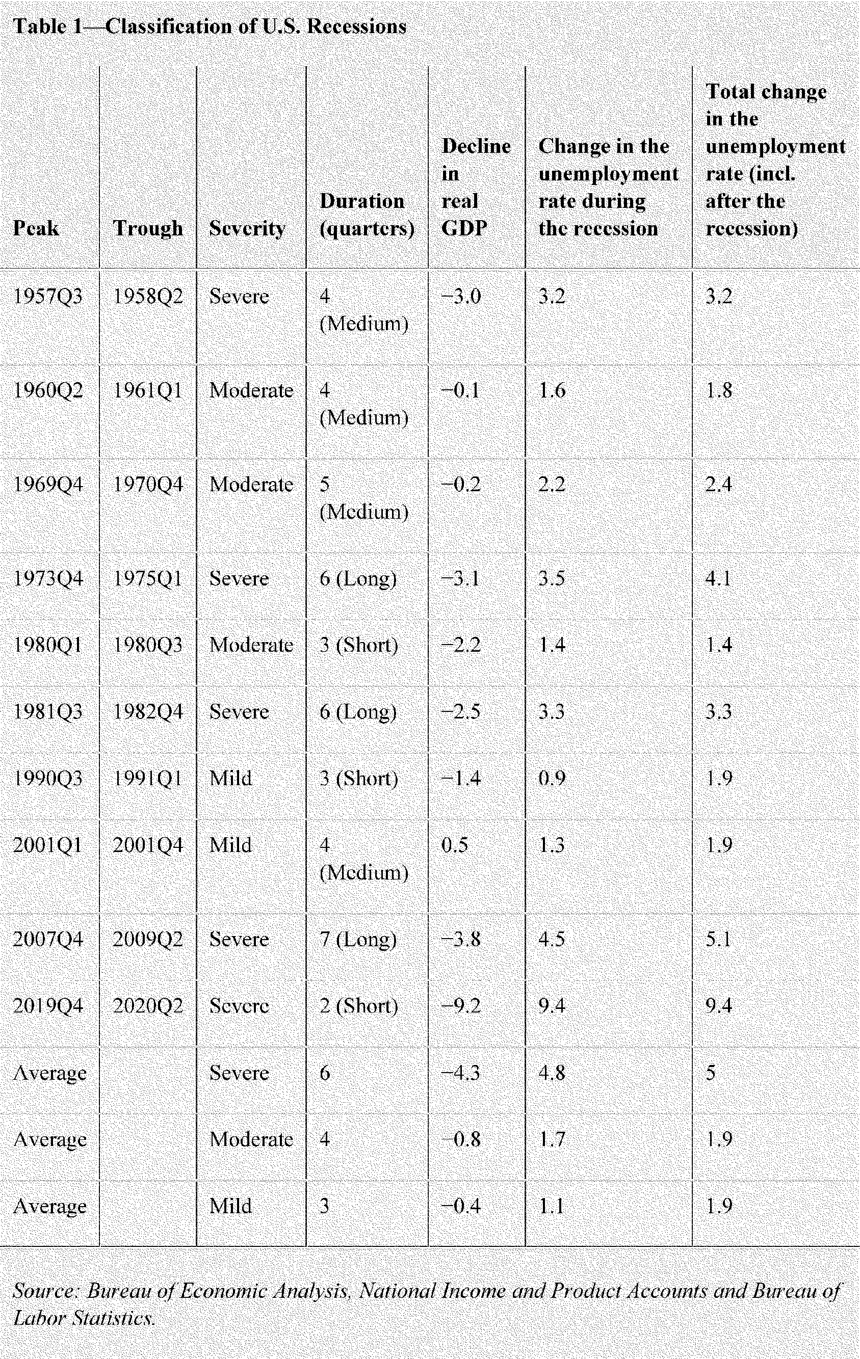

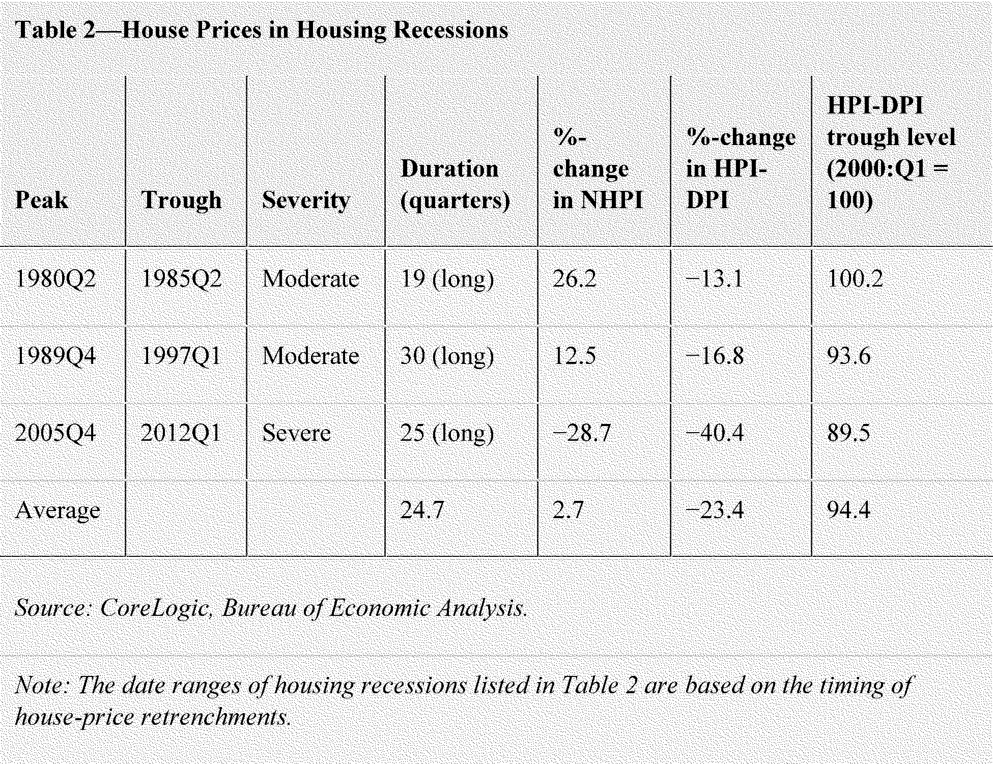
Appendix B to Part 252—Stress Testing Policy Statement

19. To amend appendix B to part 252:

a. Add paragraph (a)(iv) to section 2.1;

b. Revise section 2.2;

c. Remove the text “and non-public information about” from section 3.1;

d. Revise paragraph (c) of section 3.2.

The revisions read as follows:

2.1 Soundness in Model Design

(a) During development, the Federal Reserve

(i) subjects supervisory models to extensive review of model theory and logic and general conceptual soundness;

(ii) examines and evaluates justifications for modeling assumptions;

(iii) tests models to establish the accuracy and stability of the estimates and forecasts that they produce; and

(iv) invites, evaluates, and responds to substantive public input on material model changes.

2.2. Disclosure of Information Related to the Supervisory Stress Test

(a) In general, the Board does not disclose information related to the supervisory stress test to covered companies if that information is not also publicly disclosed. However, the Board will generally provide additional information directly to a covered company about such covered company's supervisory stress test results, provided that the Board will only do so if it provides the same type of information to all other covered companies participating in the same stress test cycle.

(b) The Board has increased the breadth of its public disclosure since the inception of the supervisory stress test to include comprehensive descriptions of the supervisory stress models, changes to those models, and, for each supervisory stress test cycle, more information about model changes and key risk drivers, in addition to more detail on different components of projected net revenues and losses. Increasing public disclosure can help the public understand and interpret the results of the supervisory stress test, particularly with respect to the condition and capital adequacy of participating firms. Providing additional information about the supervisory stress test allows the public to make an evaluation of the quality of the Board's assessment. This policy also promotes consistent and equitable treatment of covered companies by ensuring that institutions do not have access to information about the supervisory stress test that is not also accessible to other covered companies, corresponding to the principle of consistency and comparability.

3.1. Structural Independence

(b) In addition, the Model Validation Council, a council of external academic experts, provides independent advice on the Federal Reserve's process to assess models used in the supervisory stress test. In biannual meetings with Federal Reserve officials, members of the council discuss selective supervisory models, after being provided with detailed model documentation for those models. The documentation and discussions enable the council to assess the effectiveness of the models used in the supervisory stress tests and of the overarching model validation program.

3.2. Technical Competence of Validation Staff

(c) The model validation program covers three main areas of validation:

(1) Conceptual soundness;

(2) ongoing monitoring; and

(3) outcomes analysis. ( printed page 51953)

Validation staff evaluates all aspects of model development, implementation, and use, including but not limited to theory, design, methodology, input data, testing, performance, documentation standards, implementation controls (including access and change controls), and code verification.

BILLING CODE 6210-01-P

BILLING CODE 6210-01-C

[FR Doc. 2025-20211 Filed 11-17-25; 8:45 am]